19 Solutions to exercises

19.1 Chapter 3

For annual values, see 19.1:

data_ml %>%
    group_by(date) %>%                                            
    mutate(growth = Pb > median(Pb)) %>%            # Creates the sort
    ungroup() %>%                                   # Ungroup
    mutate(year = lubridate::year(date)) %>%        # Creates a year variable
    group_by(year, growth) %>%                      # Analyze by year & sort
    summarize(ret = mean(R1M_Usd)) %>%              # Compute average return
    ggplot(aes(x = year, y = ret, fill = growth)) + geom_col(position = "dodge") + # Plot!
    theme(legend.position = c(0.7, 0.8)) + theme_bw()
The value factor: annual returns.

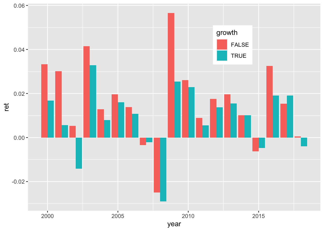
FIGURE 19.1: The value factor: annual returns.

For monthly values, see 19.2:

returns_m <- data_ml %>%
    group_by(date) %>%                                            
    mutate(growth = Pb > median(Pb)) %>%                         # Creates the sort
    group_by(date, growth) %>%                                   # Analyze by date & sort
    summarize(ret = mean(R1M_Usd)) %>%                           # Compute average return
    spread(key = growth, value = ret) %>%                        # Pivot to wide matrix format
    ungroup()
colnames(returns_m)[2:3] <- c("value", "growth")                 # Changing column names
returns_m %>%
    mutate(value = cumprod(1 + value),                           # From returns to portf. values
           growth = cumprod(1 + growth)) %>%
    gather(key = portfolio, value = value, -date) %>%            # Back in tidy format
    ggplot(aes(x = date, y = value, color = portfolio)) + geom_line() +     # Plot!  
    theme(legend.position = c(0.7, 0.8)) + theme_bw()
The value factor: portfolio values.

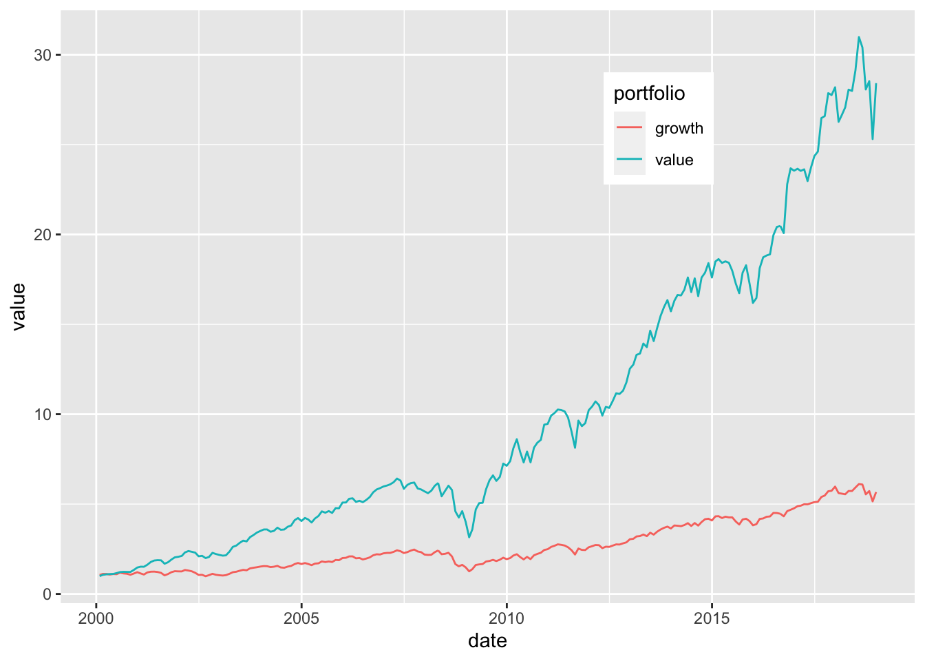
FIGURE 19.2: The value factor: portfolio values.

Portfolios based on quartiles, using the tidyverse only. We rely heavily on the fact that features are uniformized, i.e., that their distribution is uniform for each given date. Overall, small firms outperform heavily (see Figure 19.3).

data_ml %>%
    mutate(small = Mkt_Cap_6M_Usd <= 0.25,                        # Small firms...
           medium = Mkt_Cap_6M_Usd > 0.25 & Mkt_Cap_6M_Usd <= 0.5, 
           large = Mkt_Cap_6M_Usd > 0.5 & Mkt_Cap_6M_Usd <= 0.75,
           xl = Mkt_Cap_6M_Usd > 0.75,                            # ...Xlarge firms
           year = year(date)) %>%                        
    group_by(year) %>%
    summarize(small = mean(small * R1M_Usd),                      # Compute avg returns
              medium = mean(medium * R1M_Usd),
              large = mean(large * R1M_Usd),
              xl = mean(xl * R1M_Usd)) %>%
    gather(key = size, value = return, -year) %>%
    ggplot(aes(x = year, y = return, fill = size)) + 
    geom_col(position = "dodge") + theme_bw()
The value factor: portfolio values.

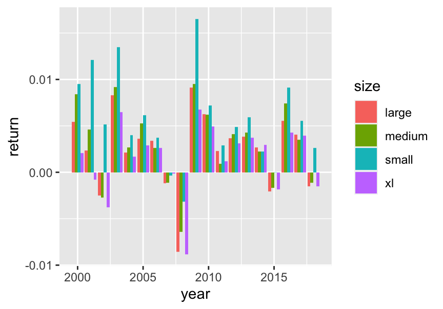
FIGURE 19.3: The value factor: portfolio values.

19.2 Chapter 4

Below, we import a credit spread supplied by Bank of America. Its symbol/ticker is “BAMLC0A0CM”. We apply the data expansion on the small number of predictors to save memory space. One important trick that should not be overlooked is the uniformization step after the product (4.3) is computed. Indeed, we want the new features to have the same properties as the old ones. If we skip this step, distributions will be altered, as we show in one example below.

We start with the data extraction and joining. It’s important to join early so as to keep the highest data frequency (daily) in order to replace missing points with close values. Joining with monthly data before replacing creates unnecessary lags.

getSymbols.FRED("BAMLC0A0CM",                                    # Extract data
                env = ".GlobalEnv", 
                return.class = "xts")
## [1] "BAMLC0A0CM"
cred_spread <- fortify(BAMLC0A0CM)                               # Transform to dataframe
colnames(cred_spread) <- c("date", "spread")                     # Change column name
cred_spread <- cred_spread %>%                                   # Take extraction and...
    full_join(data_ml %>% dplyr::select(date), by = "date") %>%  # Join!
    mutate(spread = na.locf(spread))                             # Replace NA by previous
cred_spread <- cred_spread[!duplicated(cred_spread),]            # Remove duplicates

The creation of the augmented dataset requires some manipulation. Features are no longer uniform as is shown in Figure 19.4.

data_cond <- data_ml %>%                                    # Create new dataset
    dplyr::select(c("stock_id", "date", features_short))
names_cred_spread <- paste0(features_short, "_cred_spread") # New column names
feat_cred_spread <- data_cond %>%                           # Old values
    dplyr::select(features_short)
cred_spread <- data_ml %>%                                  # Create vector of spreads
    dplyr::select(date) %>%
    left_join(cred_spread, by = "date") 
feat_cred_spread <- feat_cred_spread *                      # This product creates...
    matrix(cred_spread$spread,                              # the new values...
           length(cred_spread$spread),                      # using duplicated...
           length(features_short))                          # columns
colnames(feat_cred_spread) <- names_cred_spread             # New column names
data_cond <- bind_cols(data_cond, feat_cred_spread)         # Aggregate old & new
data_cond %>% ggplot(aes(x = Eps_cred_spread)) + geom_histogram() # Plot example
Distribution of Eps after conditioning.

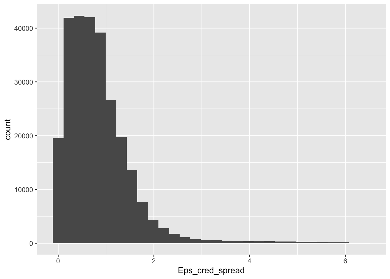
FIGURE 19.4: Distribution of Eps after conditioning.

To prevent this issue, uniformization is required and is verified in Figure 19.5.

data_cond <- data_cond %>%                   # From new dataset
    group_by(date) %>%                       # Group by date and...
    mutate_at(names_cred_spread, norm_unif)  # Uniformize the new features
data_cond %>% ggplot(aes(x = Eps_cred_spread)) + geom_histogram(bins = 100) # Verification
Distribution of uniformized conditioned feature values.

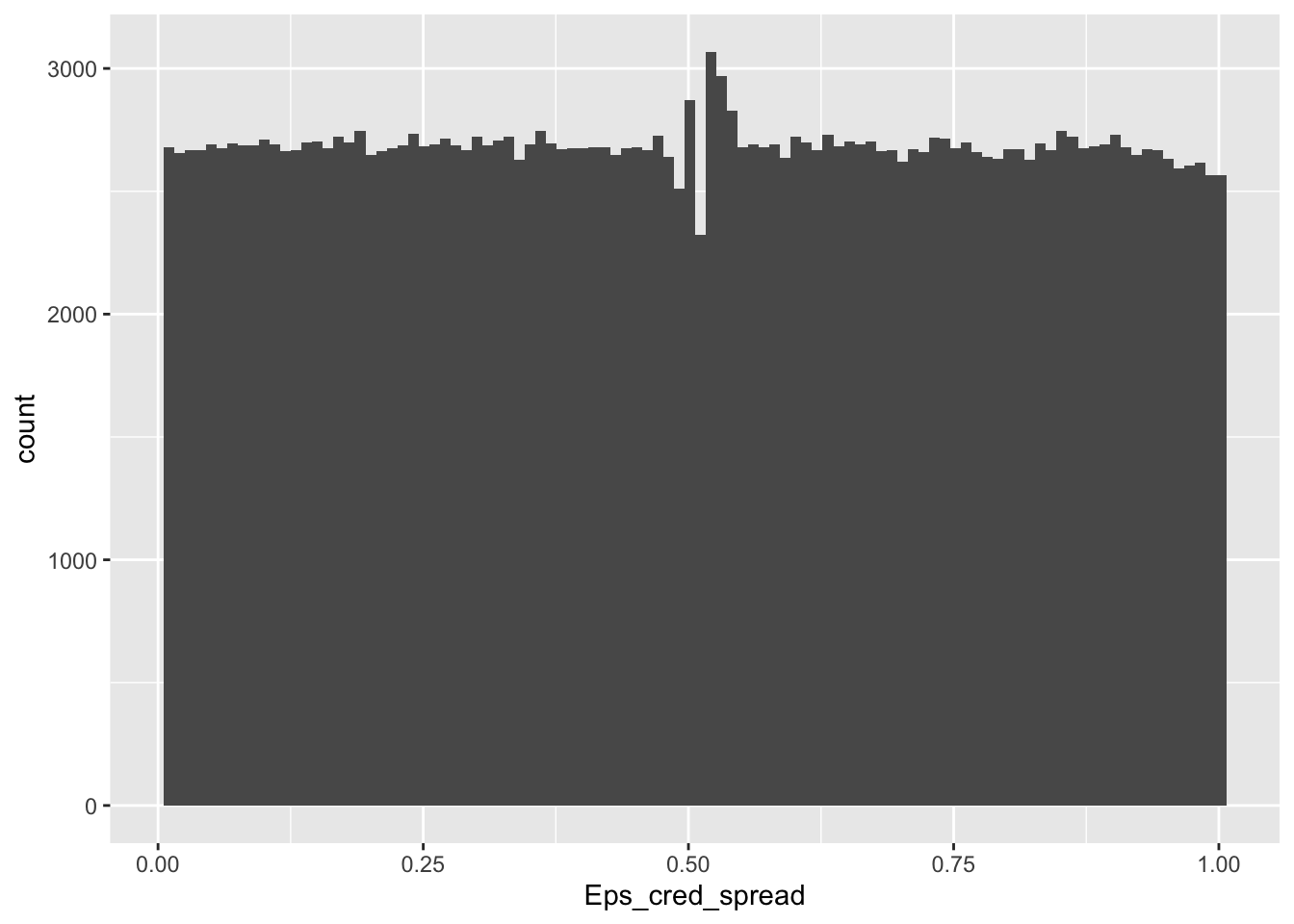
FIGURE 19.5: Distribution of uniformized conditioned feature values.

The second question naturally requires the downloading of VIX series first and the joining with the original data.

getSymbols.FRED("VIXCLS",                           # Extract data
                env = ".GlobalEnv", 
                return.class = "xts")
## [1] "VIXCLS"
vix <- fortify(VIXCLS)                              # Transform to dataframe
colnames(vix) <- c("date", "vix")                   # Change column name
vix <- vix %>%                                      # Take extraction and...
    full_join(data_ml %>% dplyr::select(date), by = "date") %>%    # Join! 
    mutate(vix = na.locf(vix))                      # Replace NA by previous
vix <- vix[!duplicated(vix),]                       # Remove duplicates
vix <- data_ml %>%                                  # Keep original data format
    dplyr::select(date) %>%                         # ...
    left_join(vix, by = "date")                     # Via left_join()

We can then proceed with the categorization. We create the vector label in a new (smaller) dataset but not attached to the large data_ml variable. Also, we check the balance of labels and its evolution through time (see Figure 19.6).

delta <- 0.5                                       # Magnitude of vix correction
vix_bar <- median(vix$vix)                         # Median of vix
data_vix <- data_ml %>%                            # Smaller dataset
    dplyr::select(stock_id, date, R1M_Usd) %>%
    mutate(r_minus = (-0.02) * exp(-delta*(vix$vix-vix_bar)),  # r_-
           r_plus = 0.02 * exp(delta*(vix$vix-vix_bar)))       # r_+
data_vix <- data_vix %>% 
    mutate(R1M_Usd_Cvix = if_else(R1M_Usd < r_minus, -1,       # New label!
                                  if_else(R1M_Usd > r_plus, 1,0)),
           R1M_Usd_Cvix = as.factor(R1M_Usd_Cvix))
data_vix %>% 
    mutate(year = year(date)) %>%
    group_by(year, R1M_Usd_Cvix) %>%
    summarize(nb = n()) %>%
    ggplot(aes(x = year, y = nb, fill = R1M_Usd_Cvix)) + 
    geom_col() + theme_bw()
Evolution of categories through time.

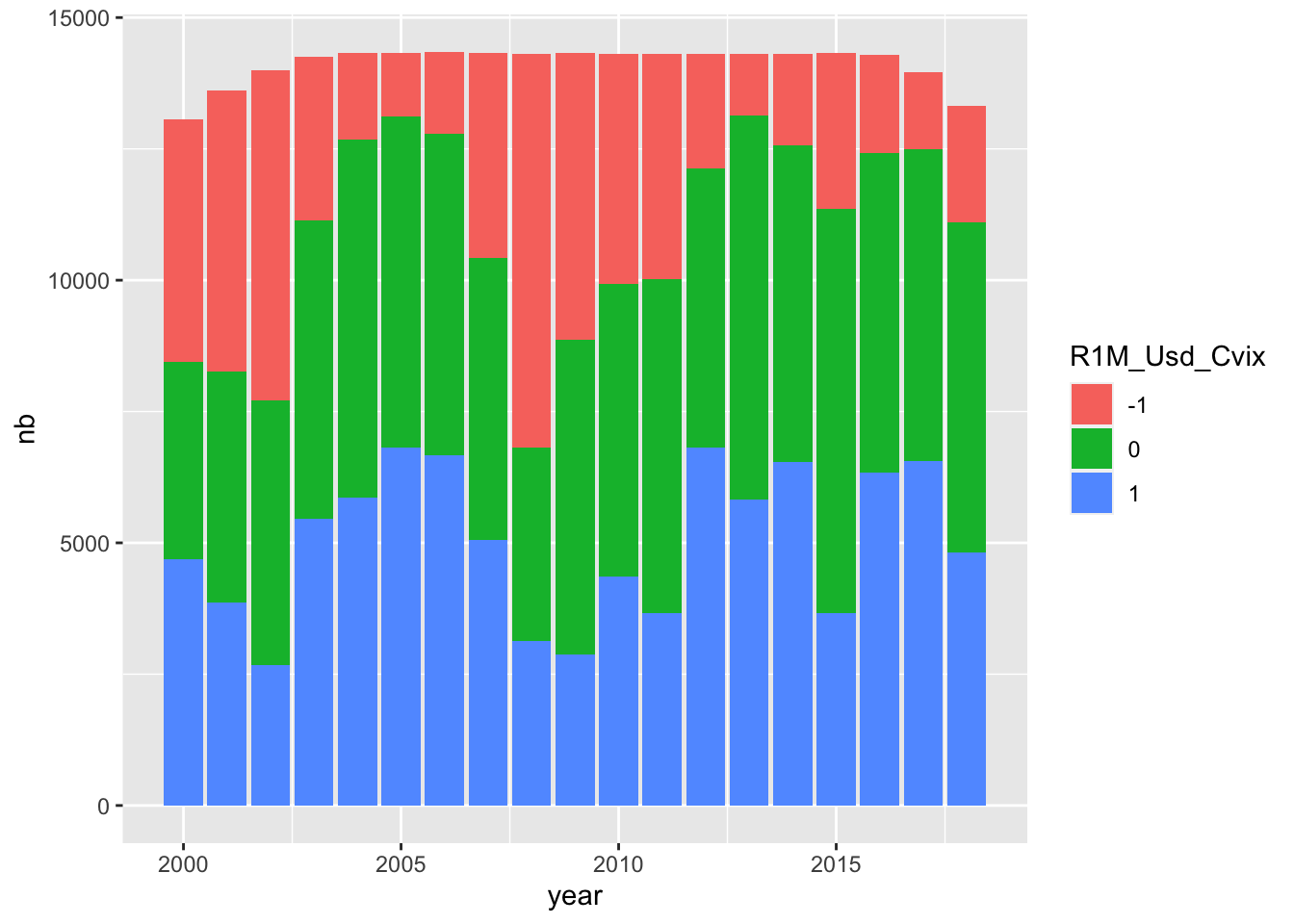
FIGURE 19.6: Evolution of categories through time.

Finally, we switch to the outliers (Figure 19.7).

data_ml %>%
    ggplot(aes(x = R12M_Usd)) + geom_histogram() + theme_bw()
Outliers in the dependent variable.

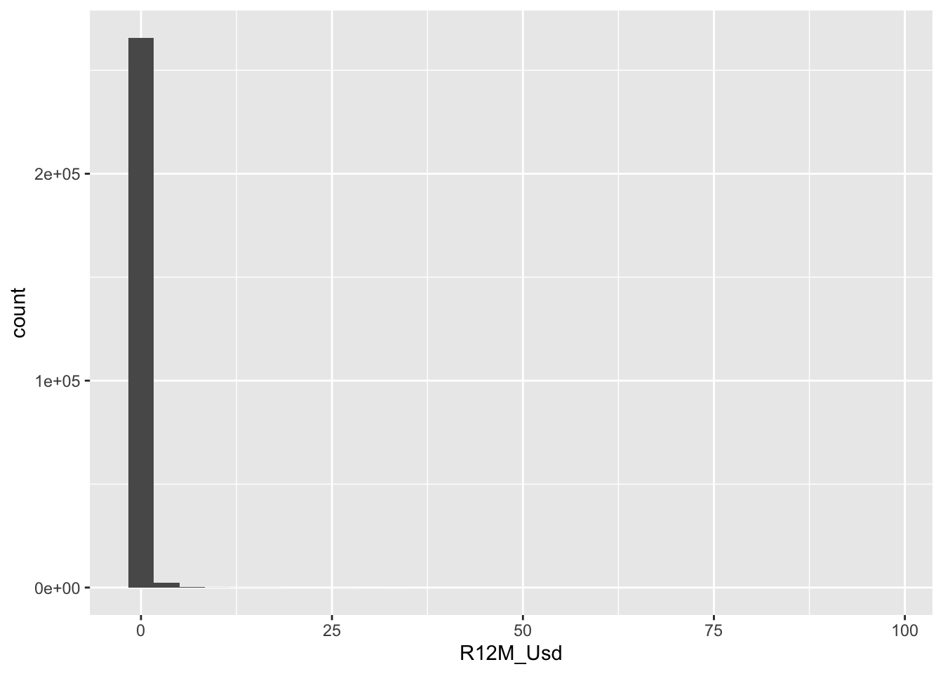
FIGURE 19.7: Outliers in the dependent variable.

Returns above 50 should indeed be rare.

data_ml %>% filter(R12M_Usd > 50) %>% dplyr::select(stock_id, date, R12M_Usd)
## # A tibble: 8 × 3
##   stock_id date       R12M_Usd
##      <int> <date>        <dbl>
## 1      212 2000-12-31     53.0
## 2      221 2008-12-31     53.5
## 3      221 2009-01-31     55.2
## 4      221 2009-02-28     54.8
## 5      296 2002-06-30     72.2
## 6      683 2009-02-28     96.0
## 7      683 2009-03-31     64.8
## 8      862 2009-02-28     58.0

The largest return comes from stock #683. Let’s have a look at the stream of monthly returns in 2009.

data_ml %>% 
    filter(stock_id == 683, year(date) == 2009) %>% 
    dplyr::select(date, R1M_Usd)
## # A tibble: 12 × 2
##    date       R1M_Usd
##    <date>       <dbl>
##  1 2009-01-31  -0.625
##  2 2009-02-28   0.472
##  3 2009-03-31   1.44 
##  4 2009-04-30   0.139
##  5 2009-05-31   0.086
##  6 2009-06-30   0.185
##  7 2009-07-31   0.363
##  8 2009-08-31   0.103
##  9 2009-09-30   9.91 
## 10 2009-10-31   0.101
## 11 2009-11-30   0.202
## 12 2009-12-31  -0.251

The returns are all very high. The annual value is plausible. In addition, a quick glance at the Vol1Y values shows that the stock is the most volatile of the dataset.

19.3 Chapter 5

We recycle the training and testing data variables created in the chapter (coding section notably). In addition, we create a dedicated function and resort to the map2() function from the purrr package.

alpha_seq <- (0:10)/10                     # Sequence of alpha values
lambda_seq <- 0.1^(0:5)                    # Sequence of lambda values
pars <- expand.grid(alpha_seq, lambda_seq) # Exploring all combinations!
alpha_seq <- pars[,1]
lambda_seq <- pars[,2]
lasso_sens <- function(alpha, lambda, x_train, y_train, x_test, y_test){ # Function
    fit_temp <- glmnet(x_train, y_train,                                 # Model
                       alpha = alpha, lambda = lambda)
    return(sqrt(mean((predict(fit_temp, x_test) - y_test)^2)))           # Output
}
rmse_elas <- map2(alpha_seq, lambda_seq, lasso_sens,                     # Automation
                  x_train = x_penalized_train, y_train = y_penalized_train,
                  x_test = x_penalized_test, y_test = testing_sample$R1M_Usd)

bind_cols(alpha = alpha_seq, lambda = as.factor(lambda_seq), rmse = unlist(rmse_elas)) %>%
    ggplot(aes(x = alpha, y = rmse, fill = lambda)) + geom_col() + facet_grid(lambda ~.) +
    coord_cartesian(ylim = c(0.19,0.193)) + theme_bw()
Performance of elasticnet across parameter values.

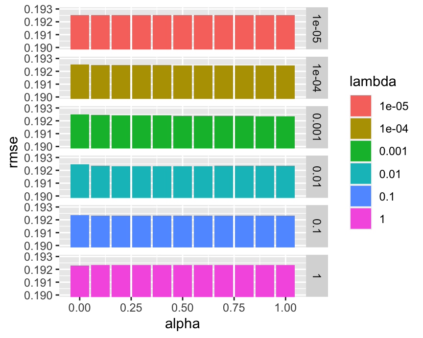
FIGURE 19.8: Performance of elasticnet across parameter values.

As is outlined in Figure 19.8, the parameters have a very marginal impact. Maybe the model is not a good fit for the task.

19.4 Chapter 6

fit1 <- rpart(formula, 
              data = training_sample,     # Data source: full sample
              cp = 0.001)                 # Precision: smaller = more leaves
mean((predict(fit1, testing_sample) - testing_sample$R1M_Usd)^2) 
## [1] 0.04018973
fit2 <- rpart(formula,
              data = training_sample,     # Data source: full sample
              cp = 0.01)                  # Precision: smaller = more leaves
mean((predict(fit2, testing_sample) - testing_sample$R1M_Usd)^2) # Test!
## [1] 0.03699696
rpart.plot(fit1)                         # Plot the first tree
Sample (complex) tree.

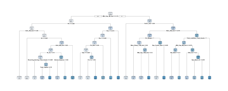
FIGURE 19.9: Sample (complex) tree.

The first model (Figure 19.9) is too precise: going into the details of the training sample does not translate to good performance out-of-sample. The second, simpler model, yields better results.

n_trees <- c(10, 20, 40, 80, 160)
mse_RF <- 0
for(j in 1:length(n_trees)){       # No need for functional programming here...
    fit_temp <- randomForest(
        as.formula(paste("R1M_Usd ~", paste(features_short, collapse = " + "))),  # New formula!
        data = training_sample,    # Data source: training sample
        sampsize = 30000,          # Size of (random) sample for each tree
        replace = TRUE,            # Is the sampling done with replacement?
        ntree = n_trees[j],        # Nb of random trees
        mtry = 5)                  # Nb of predictors for each tree
    mse_RF[j] <- mean((predict(fit_temp, testing_sample) - testing_sample$R1M_Usd)^2)
}
mse_RF
## [1] 0.03967754 0.03885924 0.03766900 0.03696370 0.03699772

Trees are by definition random so results can vary from test to test. Overall, large numbers of trees are preferable and the reason is that each new tree tells a new story and diversifies the risk of the whole forest. Some more technical details of why that may be the case are outlined in the original paper by Breiman (2001).

For the last exercises, we recycle the formula used in Chapter 6.

tree_2008 <- rpart(formula,
                   data = data_ml %>% filter(year(date) == 2008), # Data source: 2008
                   cp = 0.001,
                   maxdepth = 2) 
rpart.plot(tree_2008)
Tree for 2008.

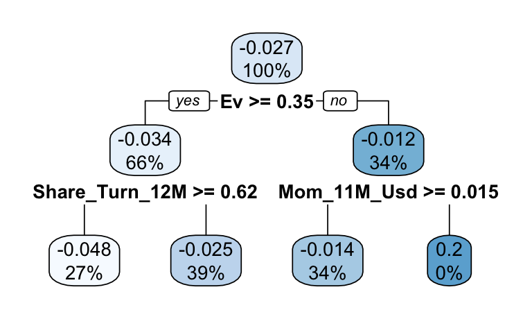
FIGURE 19.10: Tree for 2008.

The first splitting criterion in Figure 19.10 is enterprise value (EV). EV is an indicator that adjusts market capitalization by substracting debt and adding cash. It is a more faithful account of the true value of a company. In 2008, the companies that fared the least poorly were those with the highest EV (i.e., large, robust firms).

tree_2009 <- rpart(formula,
                   data = data_ml %>% filter(year(date) == 2009), # Data source: 2009
                   cp = 0.001,
                   maxdepth = 2) 
rpart.plot(tree_2009)
Tree for 2009.

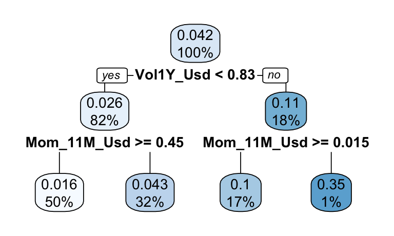
FIGURE 19.11: Tree for 2009.

In 2009 (Figure 19.11), the firms that recovered the fastest were those that experienced high volatility in the past (likely, downwards volatility). Momentum is also very important: the firms with the lowest past returns are those that rebound the fastest. This is a typical example of the momentum crash phenomenon studied in Barroso and Santa-Clara (2015) and K. Daniel and Moskowitz (2016). The rationale is the following: after a market downturn, the stocks with the most potential for growth are those that have suffered the largest losses. Consequently, the negative (short) leg of the momentum factor performs very well, often better than the long leg. And indeed, being long in the momentum factor in 2009 would have generated negative profits.

19.5 Chapter 7: the autoencoder model & universal approximation

First, it is imperative to format the inputs properly. To avoid any issues, we work with perfectly rectangular data and hence restrict the investment set to the stocks with no missing points. Dimensions must also be in the correct order.

data_short <- data_ml %>%         # Shorter dataset
    filter(stock_id %in% stock_ids_short) %>%
    dplyr::select(c("stock_id", "date",features_short, "R1M_Usd"))
dates <- unique(data_short$date)  # Vector of dates

N <- length(stock_ids_short)      # Dimension for assets
Tt <- length(dates)               # Dimension for dates
K <- length(features_short)       # Dimension for features

factor_data <- data_short %>%  # Factor side date
    dplyr::select(date, stock_id, R1M_Usd) %>%
    spread(key = stock_id, value = R1M_Usd) %>%
    dplyr::select(-date) %>%
    as.matrix()

beta_data <- array(unlist(data_short %>%  # Beta side data: beware the permutation below!
                              dplyr::select(-stock_id, -date, -R1M_Usd)), 
                   dim = c(N, Tt, K))
beta_data <- aperm(beta_data, c(2,1,3))   # Permutation

Next, we turn to the specification of the network, using a functional API form.

main_input <- layer_input(shape = c(N), name = "main_input")  # Main input: returns      
factor_network <- main_input %>%                              # Def of factor side network
    layer_dense(units = 8, activation = "relu", name = "layer_1_r") %>%
    layer_dense(units = 4, activation = "tanh", name = "layer_2_r") 

aux_input <- layer_input(shape = c(N,K), name = "aux_input")  # Aux input: characteristics
beta_network <- aux_input %>%                                 # Def of beta side network
    layer_dense(units = 8, activation = "relu", name = "layer_1_l") %>%
    layer_dense(units = 4, activation = "tanh", name = "layer_2_l") %>%
    layer_permute(dims = c(2,1), name = "layer_3_l")          # Permutation!

main_output <- layer_dot(c(beta_network, factor_network),     # Product of 2 networks
                         axes = 1, name = "main_output") 

model_ae <- keras_model(                                      # AE Model specs
    inputs = c(main_input, aux_input),
    outputs = c(main_output)
)

Finally, we ask for the structure of the model, and train it.

summary(model_ae)                      # See model details / architecture
## Model: "model_1"
## __________________________________________________________________________________________
## Layer (type)                 Output Shape        Param #    Connected to                  
## ==========================================================================================
## aux_input (InputLayer)       [(None, 793, 7)]    0                                        
## __________________________________________________________________________________________
## layer_1_l (Dense)            (None, 793, 8)      64         aux_input[0][0]               
## __________________________________________________________________________________________
## main_input (InputLayer)      [(None, 793)]       0                                        
## __________________________________________________________________________________________
## layer_2_l (Dense)            (None, 793, 4)      36         layer_1_l[0][0]               
## __________________________________________________________________________________________
## layer_1_r (Dense)            (None, 8)           6352       main_input[0][0]              
## __________________________________________________________________________________________
## layer_3_l (Permute)          (None, 4, 793)      0          layer_2_l[0][0]               
## __________________________________________________________________________________________
## layer_2_r (Dense)            (None, 4)           36         layer_1_r[0][0]               
## __________________________________________________________________________________________
## main_output (Dot)            (None, 793)         0          layer_3_l[0][0]               
##                                                             layer_2_r[0][0]               
## ==========================================================================================
## Total params: 6,488
## Trainable params: 6,488
## Non-trainable params: 0
## __________________________________________________________________________________________
model_ae %>% keras::compile(           # Learning parameters
    optimizer = "rmsprop",
    loss = "mean_squared_error"
)

model_ae %>% fit(                      # Learning function
    x = list(main_input = factor_data, aux_input = beta_data),
    y = list(main_output = factor_data),
    epochs = 20,                      # Nb rounds
    batch_size = 49                   # Nb obs. per round
)

For the second exercise, we use a simple architecture. The activation function, number of epochs and batch size may matter…

model_ua <- keras_model_sequential()
model_ua %>%   # This defines the structure of the network, i.e. how layers are organized
    layer_dense(units = 16, activation = 'sigmoid', input_shape = 1) %>%
    layer_dense(units = 1) # 
model_ua %>% keras::compile(                      # Model specification
    loss = 'mean_squared_error',                  # Loss function
    optimizer = optimizer_rmsprop(),              # Optimisation method (weight updating)
    metrics = c('mean_absolute_error')            # Output metric
)
summary(model_ua)                                 # A simple model!
## Model: "sequential_7"
## __________________________________________________________________________________________
## Layer (type)                            Output Shape                        Param #       
## ==========================================================================================
## dense_22 (Dense)                        (None, 16)                          32            
## __________________________________________________________________________________________
## dense_21 (Dense)                        (None, 1)                           17            
## ==========================================================================================
## Total params: 49
## Trainable params: 49
## Non-trainable params: 0
## __________________________________________________________________________________________
fit_ua <- model_ua %>% 
    fit(seq(0, 6, by = 0.001) %>% matrix(ncol = 1),              # Training data = x
        sin(seq(0, 6, by = 0.001)) %>% matrix(ncol = 1),         # Training label = y
        epochs = 30, batch_size = 64                             # Training parameters
) 

In full disclosure, to improve the fit, we also increase the sample size. We show the improvement in the figure below.

library(patchwork)
model_ua2 <- keras_model_sequential()
model_ua2 %>%   # This defines the structure of the network, i.e. how layers are organized
    layer_dense(units = 128, activation = 'sigmoid', input_shape = 1) %>%
    layer_dense(units = 1) # 
model_ua2 %>% keras::compile(                     # Model specification
    loss = 'mean_squared_error',                  # Loss function
    optimizer = optimizer_rmsprop(),              # Optimisation method (weight updating)
    metrics = c('mean_absolute_error')            # Output metric
)
summary(model_ua2)                                 # A simple model!
## Model: "sequential_8"
## __________________________________________________________________________________________
## Layer (type)                            Output Shape                        Param #       
## ==========================================================================================
## dense_24 (Dense)                        (None, 128)                         256           
## __________________________________________________________________________________________
## dense_23 (Dense)                        (None, 1)                           129           
## ==========================================================================================
## Total params: 385
## Trainable params: 385
## Non-trainable params: 0
## __________________________________________________________________________________________
fit_ua2 <- model_ua2 %>% 
    fit(seq(0, 6, by = 0.0002) %>% matrix(ncol = 1),            # Training data = x
        sin(seq(0, 6, by = 0.0002)) %>% matrix(ncol = 1),       # Training label = y
        epochs = 60, batch_size = 64                            # Training parameters
) 
tibble(x = seq(0, 6, by = 0.001)) %>%
  ggplot() + 
  geom_line(aes(x = x, y = predict(model_ua, x), color = "Small model")) +
  geom_line(aes(x = x, y = predict(model_ua2, x), color = "Large model")) +
  stat_function(fun = sin, aes(color = "sin(x) function")) + 
  scale_color_manual(values = c("#EEAA33", "#3366CC", "#000000")) + theme_bw()
Case with 128 units. The sine function in light blue and approximation in black.

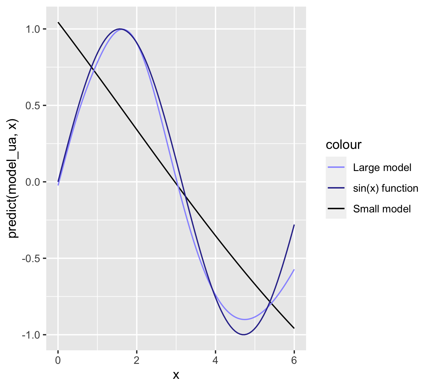
FIGURE 19.12: Case with 128 units. The sine function in light blue and approximation in black.

19.6 Chapter 8

Since we are going to reproduce a similar analysis several times, let’s simplify the task with 2 tips. First, by using default parameter values that will be passed as common arguments to the svm function. Second, by creating a custom function that computes the MSE. Third, by resorting to functional calculus via the map function from the purrr package. Below, we recycle datasets created in Chapter 6.

mse <- function(fit, features, label){             # MSE function
    return(mean((predict(fit, features)-label)^2))
}
par_list <- list(y = train_label_xgb[1:10000],     # From Tree chapter
                 x = train_features_xgb[1:10000,],
                 type = "eps-regression",
                 epsilon = 0.1,                    # Width of strip for errors
                 gamma = 0.5,                      # Constant in the radial kernel 
                 cost = 0.1)
svm_par <- function(kernel, par_list){             # Function for SVM fit automation
    require(e1071)
    return(do.call(svm, c(kernel = kernel, par_list))) 
}
kernels <- c("linear", "radial", "polynomial", "sigmoid") # Kernels
fit_svm_par <- map(kernels, svm_par, par_list = par_list) # SVM models
map(fit_svm_par, mse,                                     # MSEs
    features = test_feat_short,                           # From SVM chapter 
    label = testing_sample$R1M_Usd)
## [[1]]
## [1] 0.03849786
## 
## [[2]]
## [1] 0.03924576
## 
## [[3]]
## [1] 0.03951328
## 
## [[4]]
## [1] 334.8173

The first two kernels yield the best fit, while the last one should be avoided. Note that apart from the linear kernel, all other options require parameters. We have used the default ones, which may explain the poor performance of some nonlinear kernels.

Below, we train an SVM model on a training sample with all observations but that is limited to the 7 major predictors. Even with a smaller number of features, the training is time consuming.

svm_full <- svm(y = train_label_xgb,      # Train label
                x = train_features_xgb,   # Training features
                type = "eps-regression",  # SVM task type (see LIBSVM documentation)
                kernel = "linear",        # SVM kernel 
                epsilon = 0.1,            # Width of strip for errors
                cost = 0.1)               # Slack variable penalisation
test_feat_short <- dplyr::select(testing_sample,features_short)       # Test set
mean(predict(svm_full, test_feat_short) * testing_sample$R1M_Usd > 0) # Hit ratio
## [1] 0.490343

This figure is very low. Below, we test a very simple form of boosted trees, for comparison purposes.

xgb_full <- xgb.train(data = train_matrix_xgb,    # Data source 
                      eta = 0.3,                          # Learning rate
                      objective = "reg:linear",           # Objective function
                      max_depth = 4,                      # Maximum depth of trees
                      nrounds = 60                        # Number of trees used (bit low here)
)
## [14:44:45] WARNING: amalgamation/../src/objective/regression_obj.cu:188: reg:linear is now deprecated in favor of reg:squarederror.
mean(predict(xgb_full, xgb_test) * testing_sample$R1M_Usd > 0) # Hit ratio
## [1] 0.5017377

The forecasts are slightly better, but the computation time is lower. Two reasons why the models perform poorly:

  1. there are not enough predictors;
  2. the models are static: they do not adjust dynamically to macro-conditions.

19.7 Chapter 11: ensemble neural network

First, we create the three feature sets. The first one gets all multiples of 3 between 3 and 93. The second one gets the same indices, minus one, and the third one, the initial indices minus two.

feat_train_1 <- training_sample %>% dplyr::select(features[3*(1:31)]) %>%   # First set of feats
    as.matrix() 
feat_train_2 <- training_sample %>% dplyr::select(features[3*(1:31)-1]) %>% # Second set of feats
    as.matrix() 
feat_train_3 <- training_sample %>% dplyr::select(features[3*(1:31)-2]) %>% # Third set of feats
    as.matrix() 
feat_test_1 <- testing_sample %>% dplyr::select(features[3*(1:31)]) %>%     # Test features 1
    as.matrix() 
feat_test_2 <- testing_sample %>% dplyr::select(features[3*(1:31)-1]) %>%   # Test features 2
    as.matrix() 
feat_test_3 <- testing_sample %>% dplyr::select(features[3*(1:31)-2]) %>%   # Test features 3
    as.matrix() 

Then, we specify the network structure. First, the 3 independent networks, then the aggregation.

first_input <- layer_input(shape = c(31), name = "first_input")   # First input      
first_network <- first_input %>%                                  # Def of 1st network
    layer_dense(units = 8, activation = "relu", name = "layer_1") %>%
    layer_dense(units = 2, activation = 'softmax')                # Softmax for categ. output
second_input <- layer_input(shape = c(31), name = "second_input") # Second input      
second_network <- second_input %>%                                # Def of 2nd network
    layer_dense(units = 8, activation = "relu", name = "layer_2") %>%
    layer_dense(units = 2, activation = 'softmax')                # Softmax for categ. output
third_input <- layer_input(shape = c(31), name = "third_input")  # Third input      
third_network <- third_input %>%                                  # Def of 3rd network
    layer_dense(units = 8, activation = "relu", name = "layer_3") %>%
    layer_dense(units = 2, activation = 'softmax')                # Softmax for categ. output

main_output <- layer_concatenate(c(first_network, 
                                   second_network,
                                   third_network)) %>%            # Combination
    layer_dense(units = 2, activation = 'softmax', name = 'main_output')

model_ens <- keras_model(                                          # Agg. Model specs
    inputs = c(first_input, second_input, third_input),
    outputs = c(main_output)
)

Lastly, we can train and evaluate (see Figure 19.13).

summary(model_ens)                      # See model details / architecture
## Model: "model_2"
## __________________________________________________________________________________________
## Layer (type)                 Output Shape        Param #    Connected to                  
## ==========================================================================================
## first_input (InputLayer)     [(None, 31)]        0                                        
## __________________________________________________________________________________________
## second_input (InputLayer)    [(None, 31)]        0                                        
## __________________________________________________________________________________________
## third_input (InputLayer)     [(None, 31)]        0                                        
## __________________________________________________________________________________________
## layer_1 (Dense)              (None, 8)           256        first_input[0][0]             
## __________________________________________________________________________________________
## layer_2 (Dense)              (None, 8)           256        second_input[0][0]            
## __________________________________________________________________________________________
## layer_3 (Dense)              (None, 8)           256        third_input[0][0]             
## __________________________________________________________________________________________
## dense_23 (Dense)             (None, 2)           18         layer_1[0][0]                 
## __________________________________________________________________________________________
## dense_24 (Dense)             (None, 2)           18         layer_2[0][0]                 
## __________________________________________________________________________________________
## dense_25 (Dense)             (None, 2)           18         layer_3[0][0]                 
## __________________________________________________________________________________________
## concatenate (Concatenate)    (None, 6)           0          dense_23[0][0]                
##                                                             dense_24[0][0]                
##                                                             dense_25[0][0]                
## __________________________________________________________________________________________
## main_output (Dense)          (None, 2)           14         concatenate[0][0]             
## ==========================================================================================
## Total params: 836
## Trainable params: 836
## Non-trainable params: 0
## __________________________________________________________________________________________
model_ens %>% keras::compile(                  # Learning parameters
    optimizer = optimizer_adam(),
    loss = "binary_crossentropy",
    metrics = "categorical_accuracy"
)

fit_NN_ens <- model_ens %>% fit(               # Learning function
    x = list(first_input = feat_train_1, 
             second_input = feat_train_2,
             third_input = feat_train_3),
    y = list(main_output = NN_train_labels_C), # Recycled from NN Chapter
    epochs = 12,                               # Nb rounds
    batch_size = 512,                          # Nb obs. per round
    validation_data = list(list(feat_test_1, feat_test_2, feat_test_3),
                           NN_test_labels_C)
)
plot(fit_NN_ens)
Learning an integrated ensemble.

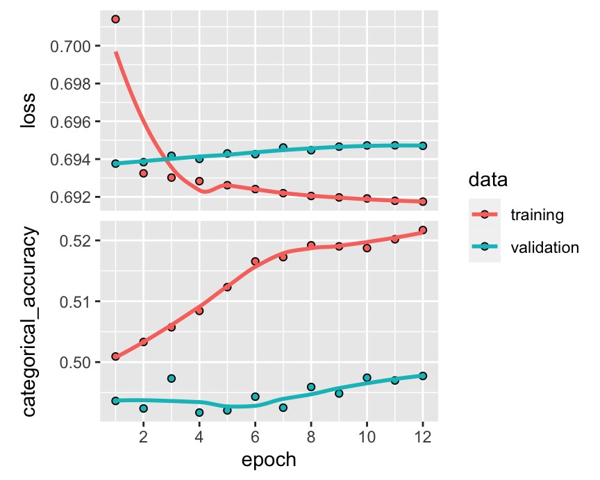
FIGURE 19.13: Learning an integrated ensemble.

19.8 Chapter 12

19.8.1 EW portfolios with the tidyverse

This one is incredibly easy; it’s simpler and more compact but close in spirit to the code that generates Figure 3.1. The returns are plotted in Figure 19.14.

data_ml %>%
  group_by(date) %>%                     # Group by date
  summarize(return = mean(R1M_Usd)) %>%  # Compute return
  ggplot(aes(x = date, y = return)) + geom_point() + geom_line() # Plot
Time series of returns.

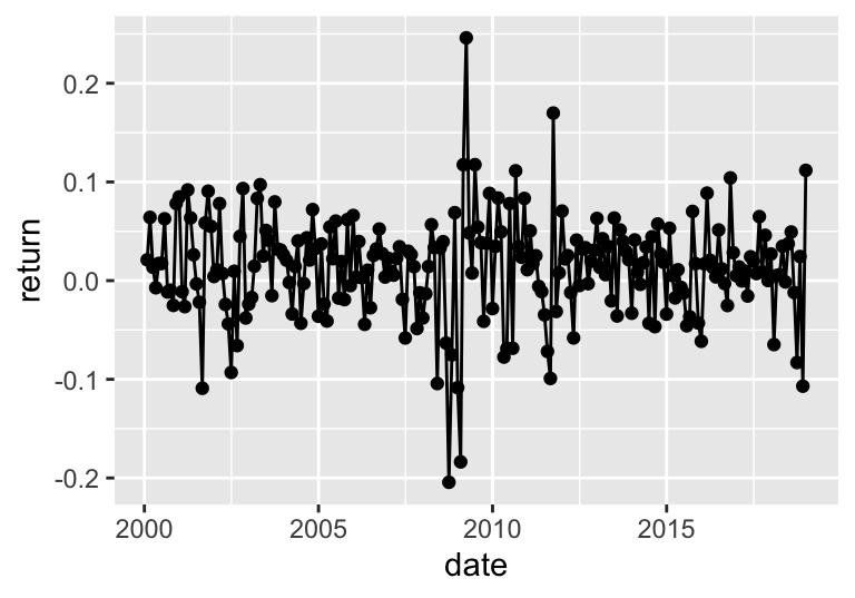
FIGURE 19.14: Time series of returns.

19.8.2 Advanced weighting function

First, we code the function with all inputs.

weights <- function(Sigma, mu, Lambda, lambda, k_D, k_R, w_old){
    N <- nrow(Sigma)
    M <- solve(lambda*Sigma + 2*k_R*Lambda + 2*k_D*diag(N)) # Inverse matrix
    num <- 1-sum(M %*% (mu + 2*k_R*Lambda %*% w_old))       # eta numerator
    den <- sum(M %*% rep(1,N))                              # eta denominator
    eta <- num / den                                        # eta
    vec <- mu + eta * rep(1,N) + 2*k_R*Lambda %*% w_old     # Vector in weight
    return(M %*% vec)
}

Second, we test it on some random dataset. We use the returns created at the end of Chapter 1 and used for the Lasso allocation in Section 5.2.2. For \(\boldsymbol{\mu}\), we use the sample average, which is rarely a good idea in practice. It serves as illustration only.

Sigma <- returns %>% dplyr::select(-date) %>% as.matrix() %>% cov()  # Covariance matrix
mu <- returns %>% dplyr::select(-date) %>% apply(2,mean)             # Vector of exp. returns
Lambda <- diag(nrow(Sigma))                                          # Trans. Cost matrix
lambda <- 1                                                          # Risk aversion
k_D <- 1
k_R <- 1
w_old <- rep(1, nrow(Sigma)) / nrow(Sigma)                           # Prev. weights: EW
weights(Sigma, mu, Lambda, lambda, k_D, k_R, w_old) %>% head()       # First weights
##             [,1]
## 1   0.0031339308
## 3  -0.0003243527
## 4   0.0011944677
## 7   0.0014194215
## 9   0.0015086240
## 11 -0.0005015207

Some weights can of course be negative. Finally, we use the map2() function to test some sensitivity. We examine 3 key indicators:
- diversification, which we measure via the inverse of the sum of squared weights (inverse Hirschman-Herfindhal index);
- leverage, which we assess via the absolute sum of negative weights;
- in-sample volatility, which we compute as \(\textbf{w}' \boldsymbol{\Sigma} \textbf{x}\)

To do so, we create a dedicated function below.

sensi <- function(lambda, k_D, Sigma, mu, Lambda, k_R, w_old){
    w <- weights(Sigma, mu, Lambda, lambda, k_D, k_R, w_old)
    out <- c()
    out$div <- 1/sum(w^2)             # Diversification
    out$lev <- sum(abs(w[w<0]))       # Leverage
    out$vol <- t(w) %*% Sigma %*% w   # In-sample vol
    return(out)
}

Instead of using the baseline map2 function, we rely on a version thereof that concatenates results into a dataframe directly.

lambda <- 10^(-3:2)              # parameter values
k_D <- 2*10^(-3:2)               # parameter values
pars <- expand_grid(lambda, k_D) # parameter grid
lambda <- pars$lambda
k_D <- pars$k_D

res <- map2_dfr(lambda, k_D, sensi, 
                Sigma = Sigma, mu = mu, Lambda = Lambda, k_R = k_R, w_old = w_old)

bind_cols(lambda = as.factor(lambda), k_D = as.factor(k_D), res) %>%
    gather(key = indicator, value = value, -lambda, -k_D) %>%
    ggplot(aes(x = lambda, y = value, fill = k_D)) + geom_col(position = "dodge") +
    facet_grid(indicator ~. , scales = "free")
Indicators related to portfolio weights.

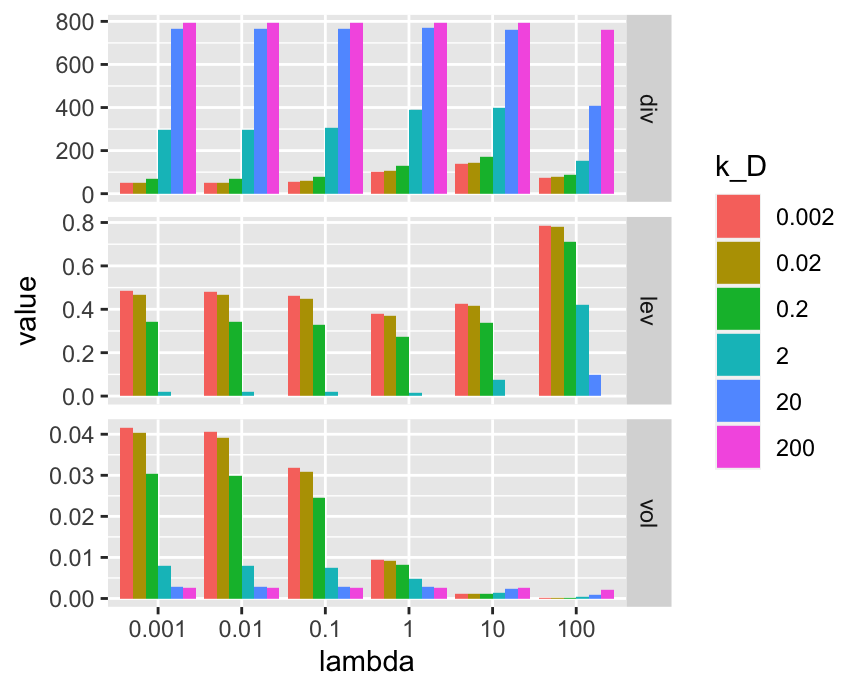
FIGURE 19.15: Indicators related to portfolio weights.

In Figure 19.15, each panel displays an indicator. In the first panel, we see that diversification increases with \(k_D\): indeed, as this number increases, the portfolio converges to uniform (EW) values. The parameter \(\lambda\) has a minor impact. The second panel naturally shows the inverse effect for leverage: as diversification increases with \(k_D\), leverage (i.e., total negative positions - shortsales) decreases. Finally, the last panel shows that in-sample volatility is however largely driven by the risk aversion parameter. As \(\lambda\) increases, volatility logically decreases. For small values of \(\lambda\), \(k_D\) is negatively related to volatility but the pattern reverses for large values of \(\lambda\). This is because the equally weighted portfolio is less risky than very leveraged mean-variance policies, but more risky than the minimum-variance portfolio.

19.8.3 Functional programming in the backtest

Often, programmers prefer to avoid loops. In order to avoid a loop in the backtest, we need to code what happens for one given date. This is encapsulated in the following function. For simplicity, we code it for only one strategy. Also, the function will assume the structure of the data is known, but the columns (features & labels) could also be passed as arguments. We recycle the function weights_xgb from Chapter 12.

portf_map <- function(t, data_ml, ticks, t_oos, m_offset, train_size, weight_func){
    train_data <- data_ml %>% filter(date < t_oos[t] - m_offset * 30,   # Roll. window w. buffer
                                     date > t_oos[t] - m_offset * 30 - 365 * train_size)
    test_data <- data_ml %>% filter(date == t_oos[t])                   # Test set  
    realized_returns <- test_data %>%                                   # Computing returns via:
        dplyr::select(R1M_Usd)                                          # 1M holding period!
    temp_weights <- weight_func(train_data, test_data, features)        # Weights = > recycled!
    ind <- match(temp_weights$names, ticks) %>% na.omit()               # Index of test assets
    x <- c() 
    x$weights <- rep(0, length(ticks))                           # Empty weights
    x$weights[ind] <- temp_weights$weights                       # Locate weights correctly
    x$returns <- sum(temp_weights$weights * realized_returns)    # Compute returns
    return(x)
}

Next, we combine this function to map(). We only test the first 6 dates: this reduces the computation times.

back_test <- 1:3 %>%             # Test on the first 100 out-of-sample dates
    map(portf_map, data_ml = data_ml, ticks = ticks, t_oos = t_oos,
        m_offset = 1, train_size = 5, weight_func = weights_xgb)
head(back_test[[1]]$weights)     # Sample weights
## [1] 0.001675042 0.000000000 0.000000000 0.001675042 0.000000000 0.001675042
back_test[[1]]$returns           # Return of first period
## [1] 0.0189129

Each element of backtest is a list with two components: the portfolio weights and the returns. To access the data easily, functions like melt from the package reshape2 are useful.

19.9 Chapter 15

We recycle the AE model trained in Chapter 15. Strangely, building smaller models (encoder) from larger ones (AE) requires to save and then reload the weights. This creates an external file, which we call “ae_weights”. We can check that the output does have 4 columns (compressed) instead of 7 (original data).

save_model_weights_hdf5(object = ae_model,filepath ="ae_weights.hdf5", overwrite = TRUE)
encoder_model <- keras_model(inputs = input_layer, outputs = encoder)
encoder_model %>% 
    load_model_weights_hdf5(filepath = "ae_weights.hdf5",skip_mismatch = TRUE,by_name = TRUE)
encoder_model %>% keras::compile(
    loss = 'mean_squared_error',
    optimizer = 'adam',
    metrics = c('mean_absolute_error')
)
encoder_model %>% 
  keras::predict_on_batch(x = training_sample %>% 
                              dplyr::select(features_short) %>% 
                              as.matrix()) %>%
    head(5)
##             [,1]     [,2]       [,3]      [,4]
## [1,] -0.08539051 1.200299 -0.8444785 -1.174033
## [2,] -0.06630807 1.195867 -0.8294346 -1.147886
## [3,] -0.09406579 1.194935 -0.8672158 -1.165673
## [4,] -0.09864470 1.191096 -0.8709179 -1.166036
## [5,] -0.10819313 1.173754 -0.8648338 -1.172021

19.10 Chapter 16

All we need to do is change the rho coefficient in the code of Chapter 16.

set.seed(42)                                                 # Fixing the random seed
n_sample <- 10^5                                             # Number of samples generated
rho <- (-0.8)                                                # Autoregressive parameter
sd <- 0.4                                                    # Std. dev. of noise
a <- 0.06 * rho                                              # Scaled mean of returns
data_RL3 <- tibble(returns = a/rho + arima.sim(n = n_sample, # Returns via AR(1) simulation
                                               list(ar = rho),       
                                               sd = sd),
                   action = round(runif(n_sample)*4)/4) %>%   # Random action (portfolio)
    mutate(new_state = if_else(returns < 0, "neg", "pos"),   # Coding of state
           reward = returns * action,                        # Reward = portfolio return
           state = lag(new_state),                           # Next state
           action = as.character(action)) %>% 
    na.omit()                                                # Remove one missing state

The learning can then proceed.

control <- list(alpha = 0.1,                        # Learning rate
                gamma = 0.7,                        # Discount factor for rewards
                epsilon = 0.1)                      # Exploration rate
fit_RL3 <- ReinforcementLearning(data_RL3,          # Main RL function
                                 s = "state", 
                                 a = "action", 
                                 r = "reward", 
                                 s_new = "new_state", 
                                 control = control)
print(fit_RL3)   # Show the output
## State-Action function Q
##          0.25         0         1      0.75       0.5
## neg 0.7107268 0.5971710 1.4662416 0.9535698 0.8069591
## pos 0.7730842 0.7869229 0.4734467 0.4258593 0.6257039
## 
## Policy
## neg pos 
## "1" "0" 
## 
## Reward (last iteration)
## [1] 3013.162

In this case, the constantly switching feature of the return process changes the outcome. The negative state is associated with large profits when the portfolio is fully invested, while the positive state has the best average reward when the agent refrains from investing.

For the second exercise, the trick is to define all possible actions, that is all combinations (+1,0-1) for the two assets on all dates. We recycle the data from Chapter 16.

pos_3 <- c(-1,0,1)                              # Possible alloc. to asset 1
pos_4 <- c(-1,0,1)                              # Possible alloc. to asset 3
pos <- expand_grid(pos_3, pos_4)                # All combinations
pos <- bind_cols(pos, id = 1:nrow(pos))         # Adding combination id

ret_pb_RL <- bind_cols(r3 = return_3, r4 = return_4, # Returns & P/B dataframe
                       pb3 = pb_3, pb4 = pb_4) 
data_RL4 <- sapply(ret_pb_RL,                        # Combining return & positions
                   rep.int, 
                   times = nrow(pos)) %>%
    data.frame() %>%
    bind_cols(id = rep(1:nrow(pos), 1, each = length(return_3))) %>%
    left_join(pos) %>% dplyr::select(-id) %>%
    mutate(action = paste(pos_3, pos_4),            # Uniting actions
           pb3 = round(5 * pb3),                    # Simplifying states
           pb4 = round(5 * pb4),                    # Simplifying states
           state = paste(pb3, pb4),                 # Uniting states
           reward = pos_3*r3 + pos_4*r4,            # Computing rewards
           new_state = lead(state)) %>%             # Infer new state
    dplyr::select(-pb3, -pb4, -pos_3,          # Remove superfluous vars.
                  -pos_4, -r3, -r4) 

We can the plug this data into the RL function.

fit_RL4 <- ReinforcementLearning(data_RL4,           # Main RL function
                                 s = "state", 
                                 a = "action", 
                                 r = "reward", 
                                 s_new = "new_state", 
                                 control = control)
fit_RL4$Q <- round(fit_RL4$Q, 3) # Round the Q-matrix
print(fit_RL4)                   # Show the output 
## State-Action function Q
##       0 0    0 1  0 -1  -1 -1   -1 0   -1 1   1 -1    1 0    1 1
## 0 2 0.000  0.000 0.002 -0.017 -0.018 -0.020  0.023  0.025  0.024
## 0 3 0.001 -0.005 0.007 -0.013 -0.019 -0.026  0.031  0.027  0.021
## 3 1 0.003  0.003 0.003  0.002  0.002  0.003  0.002  0.002  0.003
## 2 1 0.027  0.038 0.020  0.004  0.015  0.039  0.013  0.021  0.041
## 2 2 0.021  0.014 0.027  0.038  0.047  0.045 -0.004 -0.011 -0.016
## 2 3 0.007  0.006 0.008  0.054  0.057  0.056 -0.041 -0.041 -0.041
## 1 1 0.027  0.054 0.005 -0.031 -0.005  0.041  0.025  0.046  0.072
## 1 2 0.019  0.020 0.020  0.015  0.023  0.029  0.012  0.014  0.023
## 1 3 0.008  0.019 0.000 -0.036 -0.027 -0.016  0.042  0.053  0.060
## 
## Policy
##    0 2    0 3    3 1    2 1    2 2    2 3    1 1    1 2    1 3 
##  "1 0" "1 -1" "0 -1"  "1 1" "-1 0" "-1 0"  "1 1" "-1 1"  "1 1" 
## 
## Reward (last iteration)
## [1] 0

The matrix is less sparse compared to the one of Chapter 16; we have covered much more ground! Some policy recommendations have not changed compared to the smaller sample, but some have! The change occurs for the states for which only a few points were available in the first trial. With more data, the decision is altered.

Abbasi, Ahmed, Conan Albrecht, Anthony Vance, and James Hansen. 2012. “Metafraud: A Meta-Learning Framework for Detecting Financial Fraud.” MIS Quarterly, 1293–1327.
Aboussalah, Amine Mohamed, and Chi-Guhn Lee. 2020. “Continuous Control with Stacked Deep Dynamic Recurrent Reinforcement Learning for Portfolio Optimization.” Expert Systems with Applications 140: 112891.
Adler, Timothy, and Mark Kritzman. 2008. “The Cost of Socially Responsible Investing.” Journal of Portfolio Management 35 (1): 52–56.
Agarwal, Amit, Elad Hazan, Satyen Kale, and Robert E Schapire. 2006. “Algorithms for Portfolio Management Based on the Newton Method.” In Proceedings of the 23rd International Conference on Machine Learning, 9–16. ACM.
Aggarwal, Charu C. 2013. Outlier Analysis. Springer.
Akey, Pat, Adriana Robertson, and Mikhail Simutin. 2021. “Noisy Factors.” SSRN Working Paper 3930228.
Aldridge, Irene, and Marco Avellaneda. 2019. “Neural Networks in Finance: Design and Performance.” Journal of Financial Data Science 1 (4): 39–62.
Alessandrini, Fabio, and Eric Jondeau. 2020. “Optimal Strategies for ESG Portfolios.” SSRN Working Paper 3578830.
Allison, Paul D. 2001. Missing Data. Vol. 136. Sage publications.
Almahdi, Saud, and Steve Y Yang. 2017. “An Adaptive Portfolio Trading System: A Risk-Return Portfolio Optimization Using Recurrent Reinforcement Learning with Expected Maximum Drawdown.” Expert Systems with Applications 87: 267–79.
———. 2019. “A Constrained Portfolio Trading System Using Particle Swarm Algorithm and Recurrent Reinforcement Learning.” Expert Systems with Applications 130: 145–56.
Alti, Aydoğan, and Sheridan Titman. 2019. “A Dynamic Model of Characteristic-Based Return Predictability.” Journal of Finance 74 (6): 3187–3216.
Ammann, Manuel, Guillaume Coqueret, and Jan-Philip Schade. 2016. “Characteristics-Based Portfolio Choice with Leverage Constraints.” Journal of Banking & Finance 70: 23–37.
Amrhein, Valentin, Sander Greenland, and Blake McShane. 2019. “Scientists Rise up Against Statistical Significance.” Nature 567: 305–7.
Anderson, James A, and Edward Rosenfeld. 2000. Talking Nets: An Oral History of Neural Networks. MIT Press.
Andersson, Kristoffer, and Cornelis Oosterlee. 2020. “A Deep Learning Approach for Computations of Exposure Profiles for High-Dimensional Bermudan Options.” arXiv Preprint, no. 2003.01977.
André, Eric, and Guillaume Coqueret. 2020. “Dirichlet Policies for Reinforced Factor Portfolios.” SSRN Working Paper 3726714.
Ang, Andrew. 2014. Asset Management: A Systematic Approach to Factor Investing. Oxford University Press.
Ang, Andrew, Robert J Hodrick, Yuhang Xing, and Xiaoyan Zhang. 2006. “The Cross-Section of Volatility and Expected Returns.” Journal of Finance 61 (1): 259–99.
Ang, Andrew, and Dennis Kristensen. 2012. “Testing Conditional Factor Models.” Journal of Financial Economics 106 (1): 132–56.
Ang, Andrew, Jun Liu, and Krista Schwarz. 2018. “Using Individual Stocks or Portfolios in Tests of Factor Models.” SSRN Working Paper 1106463.
Arik, Sercan O, and Tomas Pfister. 2020. “TabNet: Attentive Interpretable Tabular Learning.” arXiv Preprint, no. 1908.07442.
Arjovsky, Martin, Léon Bottou, Ishaan Gulrajani, and David Lopez-Paz. 2019. “Invariant Risk Minimization.” arXiv Preprint, no. 1907.02893.
Arnott, Robert D, Mark Clements, Vitali Kalesnik, and Juhani T Linnainmaa. 2021. “Factor Momentum.” SSRN Working Paper 3116974.
Arnott, Robert D, Jason C Hsu, Jun Liu, and Harry Markowitz. 2014. “Can Noise Create the Size and Value Effects?” Management Science 61 (11): 2569–79.
Arnott, Rob, Campbell R Harvey, Vitali Kalesnik, and Juhani Linnainmaa. 2019. “Alice’s Adventures in Factorland: Three Blunders That Plague Factor Investing.” Journal of Portfolio Management 45 (4): 18–36.
Arnott, Rob, Campbell R Harvey, and Harry Markowitz. 2019. “A Backtesting Protocol in the Era of Machine Learning.” Journal of Financial Data Science 1 (1): 64–74.
Aronow, Peter M., and Fredrik Sävje. 2019. “Book Review. The Book of Why: The New Science of Cause and Effect.” Journal of the American Statistical Association 115 (529): 482–85.
Asness, Cliff, Andrea Frazzini, Niels Joachim Gormsen, and Lasse Heje Pedersen. 2020. “Betting Against Correlation: Testing Theories of the Low-Risk Effect.” Journal of Financial Economics 135 (3): 629–52.
Asness, Clifford S, Tobias J Moskowitz, and Lasse Heje Pedersen. 2013. “Value and Momentum Everywhere.” Journal of Finance 68 (3): 929–85.
Asness, Clifford, Swati Chandra, Antti Ilmanen, and Ronen Israel. 2017. “Contrarian Factor Timing Is Deceptively Difficult.” Journal of Portfolio Management 43 (5): 72–87.
Asness, Clifford, and Andrea Frazzini. 2013. “The Devil in HML’s Details.” Journal of Portfolio Management 39 (4): 49–68.
Asness, Clifford, Andrea Frazzini, Ronen Israel, Tobias J Moskowitz, and Lasse H Pedersen. 2018. “Size Matters, If You Control Your Junk.” Journal of Financial Economics 129 (3): 479–509.
Asness, Clifford, Antti Ilmanen, Ronen Israel, and Tobias Moskowitz. 2015. “Investing with Style.” Journal of Investment Management 13 (1): 27–63.
Astakhov, Anton, Tomas Havranek, and Jiri Novak. 2019. “Firm Size and Stock Returns: A Quantitative Survey.” Journal of Economic Surveys 33 (5): 1463–92.
Atta-Darkua, Vaska, David Chambers, Elroy Dimson, Zhenkai Ran, and Ting Yu. 2020. “Strategies for Responsible Investing: Emerging Academic Evidence.” Journal of Portfolio Management 46 (3): 26–35.
Babiak, Mykola, and Jozef Barunik. 2020. “Deep Learning, Predictability, and Optimal Portfolio Returns.” arXiv Preprint, no. 2009.03394.
Bache, Stefan Milton, and Hadley Wickham. 2014. “Magrittr: A Forward-Pipe Operator for r.” R Package Version 1 (1).
Back, Kerry. 2010. Asset Pricing and Portfolio Choice Theory. Oxford University Press.
Baesens, Bart, Veronique Van Vlasselaer, and Wouter Verbeke. 2015. Fraud Analytics Using Descriptive, Predictive, and Social Network Techniques: A Guide to Data Science for Fraud Detection. John Wiley & Sons.
Bai, Jushan, and Serena Ng. 2002. “Determining the Number of Factors in Approximate Factor Models.” Econometrica 70 (1): 191–221.
Bailey, David H, and Marcos Lopez de Prado. 2021. “Finance Is Not Excused: Why Finance Should Not Flout Basic Principles of Statistics.” Significance (Royal Statistical Society) Forthcoming.
Bailey, David H, and Marcos López de Prado. 2014. “The Deflated Sharpe Ratio: Correcting for Selection Bias, Backtest Overfitting, and Non-Normality.” Journal of Portfolio Management 40 (5): 39–59.
Bailey, T, and A. K. Jain. 1978. “A Note on Distance-Weighted k-Nearest Neighbor Rules.” IEEE Trans. On Systems, Man, Cybernetics 8 (4): 311–13.
Bajgrowicz, Pierre, and Olivier Scaillet. 2012. “Technical Trading Revisited: False Discoveries, Persistence Tests, and Transaction Costs.” Journal of Financial Economics 106 (3): 473–91.
Baker, Malcolm, Brendan Bradley, and Jeffrey Wurgler. 2011. “Benchmarks as Limits to Arbitrage: Understanding the Low-Volatility Anomaly.” Financial Analysts Journal 67 (1): 40–54.
Baker, Malcolm, Mathias F Hoeyer, and Jeffrey Wurgler. 2020. “Leverage and the Beta Anomaly.” Journal of Financial and Quantitative Analysis Forthcoming: 1–24.
Baker, Malcolm, Patrick Luo, and Ryan Taliaferro. 2017. “Detecting Anomalies: The Relevance and Power of Standard Asset Pricing Tests.”
Bali, Turan G, Robert F Engle, and Scott Murray. 2016. Empirical Asset Pricing: The Cross Section of Stock Returns. John Wiley & Sons.
Bali, Turan G, Amit Goyal, Dashan Huang, Fuwei Jiang, and Quan Wen. 2020. “Different Strokes: Return Predictability Across Stocks and Bonds with Machine Learning and Big Data.” SSRN Working Paper 3686164.
Ballings, Michel, Dirk Van den Poel, Nathalie Hespeels, and Ruben Gryp. 2015. “Evaluating Multiple Classifiers for Stock Price Direction Prediction.” Expert Systems with Applications 42 (20): 7046–56.
Ban, Gah-Yi, Noureddine El Karoui, and Andrew EB Lim. 2016. “Machine Learning and Portfolio Optimization.” Management Science 64 (3): 1136–54.
Bansal, Ravi, David A Hsieh, and S Viswanathan. 1993. “A New Approach to International Arbitrage Pricing.” Journal of Finance 48 (5): 1719–47.
Bansal, Ravi, and Salim Viswanathan. 1993. “No Arbitrage and Arbitrage Pricing: A New Approach.” Journal of Finance 48 (4): 1231–62.
Banz, Rolf W. 1981. “The Relationship Between Return and Market Value of Common Stocks.” Journal of Financial Economics 9 (1): 3–18.
Barberis, Nicholas. 2018. “Psychology-Based Models of Asset Prices and Trading Volume.” In Handbook of Behavioral Economics-Foundations and Applications.
Barberis, Nicholas, Robin Greenwood, Lawrence Jin, and Andrei Shleifer. 2015. X-CAPM: An Extrapolative Capital Asset Pricing Model.” Journal of Financial Economics 115 (1): 1–24.
Barberis, Nicholas, Lawrence J Jin, and Baolian Wang. 2020. “Prospect Theory and Stock Market Anomalies.” SSRN Working Paper 3477463.
Barberis, Nicholas, Abhiroop Mukherjee, and Baolian Wang. 2016. “Prospect Theory and Stock Returns: An Empirical Test.” Review of Financial Studies 29 (11): 3068–3107.
Barberis, Nicholas, and Andrei Shleifer. 2003. “Style Investing.” Journal of Financial Economics 68 (2): 161–99.
Barillas, Francisco, and Jay Shanken. 2018. “Comparing Asset Pricing Models.” Journal of Finance 73 (2): 715–54.
Barron, Andrew R. 1993. “Universal Approximation Bounds for Superpositions of a Sigmoidal Function.” IEEE Transactions on Information Theory 39 (3): 930–45.
———. 1994. “Approximation and Estimation Bounds for Artificial Neural Networks.” Machine Learning 14 (1): 115–33.
Barroso, Pedro, and Pedro Santa-Clara. 2015. “Momentum Has Its Moments.” Journal of Financial Economics 116 (1): 111–20.
Basak, Jayanta. 2004. “Online Adaptive Decision Trees.” Neural Computation 16 (9): 1959–81.
Bates, John M, and Clive WJ Granger. 1969. “The Combination of Forecasts.” Journal of the Operational Research Society 20 (4): 451–68.
Bauder, David, Taras Bodnar, Nestor Parolya, and Wolfgang Schmid. 2020. “Bayesian Inference of the Multi-Period Optimal Portfolio for an Exponential Utility.” Journal of Multivariate Analysis 175: 104544.
Baz, Jamil, Nicolas Granger, Campbell R Harvey, Nicolas Le Roux, and Sandy Rattray. 2015. “Dissecting Investment Strategies in the Cross Section and Time Series.” SSRN Working Paper 2695101.
Beery, Sara, Grant Van Horn, and Pietro Perona. 2018. “Recognition in Terra Incognita.” In Proceedings of the European Conference on Computer Vision (ECCV), 456–73.
Belle, Vaishak, and Ioannis Papantonis. 2020. “Principles and Practice of Explainable Machine Learning.” arXiv Preprint, no. 2009.11698.
Bellone, Benoit, Thomas Heckel, François Soupé, and Raul Leote de Carvalho. 2020. “Equity Factor Investing: Historical Perspective of Recent Performance.” SSRN Working Paper 3732113.
Belsley, David A, Edwin Kuh, and Roy E Welsch. 2005. Regression Diagnostics: Identifying Influential Data and Sources of Collinearity. Vol. 571. John Wiley & Sons.
Bénard, Clément, Gérard Biau, Sébastien Da Veiga, and Erwan Scornet. 2021. “Sirus: Stable and Interpretable Rule Set for Classification.” Electronic Journal of Statistics 15 (1): 427–505.
Ben-David, Shai, John Blitzer, Koby Crammer, Alex Kulesza, Fernando Pereira, and Jennifer Wortman Vaughan. 2010. “A Theory of Learning from Different Domains.” Machine Learning 79 (1-2): 151–75.
Bengio, Yoshua. 2012. “Practical Recommendations for Gradient-Based Training of Deep Architectures.” In Neural Networks: Tricks of the Trade, 437–78. Springer.
Berg, Florian, Julian F Koelbel, and Roberto Rigobon. 2020. “Aggregate Confusion: The Divergence of ESG Ratings.” SSRN Working Paper 3438533.
Bergstra, James, and Yoshua Bengio. 2012. “Random Search for Hyper-Parameter Optimization.” Journal of Machine Learning Research 13 (Feb): 281–305.
Berk, Jonathan B, Richard C Green, and Vasant Naik. 1999. “Optimal Investment, Growth Options, and Security Returns.” Journal of Finance 54 (5): 1553–1607.
Bernstein, Asaf, Matthew T Gustafson, and Ryan Lewis. 2019. “Disaster on the Horizon: The Price Effect of Sea Level Rise.” Journal of Financial Economics 134 (2): 253–72.
Bertoluzzo, Francesco, and Marco Corazza. 2012. “Testing Different Reinforcement Learning Configurations for Financial Trading: Introduction and Applications.” Procedia Economics and Finance 3: 68–77.
Bertsekas, Dimitri P. 2017. Dynamic Programming and Optimal Control - Volume II, Fourth Edition. Athena Scientific.
Betermier, Sebastien, Laurent E Calvet, and Evan Jo. 2019. “A Supply and Demand Approach to Equity Pricing.” SSRN Working Paper 3440147.
Betermier, Sebastien, Laurent E Calvet, and Paolo Sodini. 2017. “Who Are the Value and Growth Investors?” Journal of Finance 72 (1): 5–46.
Bhamra, Harjoat S, and Raman Uppal. 2019. “Does Household Finance Matter? Small Financial Errors with Large Social Costs.” American Economic Review 109 (3): 1116–54.
Bhatia, Nitin et al. 2010. “Survey of Nearest Neighbor Techniques.” arXiv Preprint, no. 1007.0085.
Bhattacharyya, Siddhartha, Sanjeev Jha, Kurian Tharakunnel, and J Christopher Westland. 2011. “Data Mining for Credit Card Fraud: A Comparative Study.” Decision Support Systems 50 (3): 602–13.
Biau, Gérard. 2012. “Analysis of a Random Forests Model.” Journal of Machine Learning Research 13 (Apr): 1063–95.
Biau, Gérard, Luc Devroye, and GAbor Lugosi. 2008. “Consistency of Random Forests and Other Averaging Classifiers.” Journal of Machine Learning Research 9 (Sep): 2015–33.
Biecek, Przemyslaw, and Tomasz Burzykowski. 2021. Explanatory Model Analysis: Explore, Explain, and Examine Predictive Models. CRC Press.
Binz, Oliver, Katherine Schipper, and Kevin Standridge. 2020. “What Can Analysts Learn from Artificial Intelligence about Fundamental Analysis?” SSRN Working Paper 3745078.
Black, Fischer, and Robert Litterman. 1992. “Global Portfolio Optimization.” Financial Analysts Journal 48 (5): 28–43.
Blank, Herbert, Richard Davis, and Shannon Greene. 2019. “Using Alternative Research Data in Real-World Portfolios.” Journal of Investing 28 (4): 95–103.
Blitz, David, and Laurens Swinkels. 2020. “Is Exclusion Effective?” Journal of Portfolio Management 46 (3): 42–48.
Blum, Avrim, and Adam Kalai. 1999. “Universal Portfolios with and Without Transaction Costs.” Machine Learning 35 (3): 193–205.
Bodnar, Taras, Nestor Parolya, and Wolfgang Schmid. 2013. “On the Equivalence of Quadratic Optimization Problems Commonly Used in Portfolio Theory.” European Journal of Operational Research 229 (3): 637–44.
Boehmke, Brad, and Brandon Greenwell. 2019. Hands-on Machine Learning with r. Chapman & Hall / CRC.
Boloorforoosh, Ali, Peter Christoffersen, Christian Gourieroux, and Mathieu Fournier. 2020. “Beta Risk in the Cross-Section of Equities.” Review of Financial Studies Forthcoming.
Bonaccolto, Giovanni, and Sandra Paterlini. 2019. “Developing New Portfolio Strategies by Aggregation.” Annals of Operations Research, 1–39.
Boriah, Shyam, Varun Chandola, and Vipin Kumar. 2008. “Similarity Measures for Categorical Data: A Comparative Evaluation.” In Proceedings of the 2008 SIAM International Conference on Data Mining, 243–54.
Borisov, Vadim, Tobias Leemann, Kathrin Seßler, Johannes Haug, Martin Pawelczyk, and Gjergji Kasneci. 2021. “Deep Neural Networks and Tabular Data: A Survey.” arXiv Preprint, no. 2110.01889.
Boser, Bernhard E, Isabelle M Guyon, and Vladimir N Vapnik. 1992. “A Training Algorithm for Optimal Margin Classifiers.” In Proceedings of the Fifth Annual Workshop on Computational Learning Theory, 144–52. ACM.
Bouchaud, Jean-philippe, Philipp Krueger, Augustin Landier, and David Thesmar. 2019. “Sticky Expectations and the Profitability Anomaly.” Journal of Finance 74 (2): 639–74.
Bouthillier, Xavier, and Gaël Varoquaux. 2020. “Survey of Machine-Learning Experimental Methods at NeurIPS2019 and ICLR2020.” Research Report. Inria Saclay Ile de France.
Boyd, Stephen, and Lieven Vandenberghe. 2004. Convex Optimization. Cambridge University Press.
Branch, Ben, and Li Cai. 2012. “Do Socially Responsible Index Investors Incur an Opportunity Cost?” Financial Review 47 (3): 617–30.
Brandt, Michael W, Pedro Santa-Clara, and Rossen Valkanov. 2009. “Parametric Portfolio Policies: Exploiting Characteristics in the Cross-Section of Equity Returns.” Review of Financial Studies 22 (9): 3411–47.
Braun, Helmut, and John S Chandler. 1987. “Predicting Stock Market Behavior Through Rule Induction: An Application of the Learning-from-Example Approach.” Decision Sciences 18 (3): 415–29.
Breiman, Leo. 1996. “Stacked Regressions.” Machine Learning 24 (1): 49–64.
———. 2001. “Random Forests.” Machine Learning 45 (1): 5–32.
Breiman, Leo et al. 2004. “Population Theory for Boosting Ensembles.” Annals of Statistics 32 (1): 1–11.
Breiman, Leo, Jerome Friedman, Charles J. Stone, and R. A. Olshen. 1984. Classification and Regression Trees. Chapman & Hall.
Briere, Marie, and Ariane Szafarz. 2021. “When It Rains, It Pours: Multifactor Asset Management in Good and Bad Times.” Journal of Financial Research Forthcoming.
Brightman, Chris, Feifei Li, and Xi Liu. 2015. “Chasing Performance with ETFs.” Research Affiliates (November).
Brodersen, Kay H, Fabian Gallusser, Jim Koehler, Nicolas Remy, Steven L Scott, et al. 2015. “Inferring Causal Impact Using Bayesian Structural Time-Series Models.” Annals of Applied Statistics 9 (1): 247–74.
Brodie, Joshua, Ingrid Daubechies, Christine De Mol, Domenico Giannone, and Ignace Loris. 2009. “Sparse and Stable Markowitz Portfolios.” Proceedings of the National Academy of Sciences 106 (30): 12267–72.
Brown, Iain, and Christophe Mues. 2012. “An Experimental Comparison of Classification Algorithms for Imbalanced Credit Scoring Data Sets.” Expert Systems with Applications 39 (3): 3446–53.
Bruder, Benjamin, Yazid Cheikh, Florent Deixonne, and Ban Zheng. 2019. “Integration of ESG in Asset Allocation.” SSRN Working Paper 3473874.
Bryzgalova, Svetlana. 2019. “Spurious Factors in Linear Asset Pricing Models.”
Bryzgalova, Svetlana, Jiantao Huang, and Christian Julliard. 2019. “Bayesian Solutions for the Factor Zoo: We Just Ran Two Quadrillion Models.” SSRN Working Paper 3481736.
Bryzgalova, Svetlana, Markus Pelger, and Jason Zhu. 2019. “Forest Through the Trees: Building Cross-Sections of Stock Returns.” SSRN Working Paper 3493458.
Buehler, Hans, Lukas Gonon, Josef Teichmann, and Ben Wood. 2019. “Deep Hedging.” Quantitative Finance 19 (8): 1271–91.
Buehler, Hans, Blanka Horvath, Terry Lyons, Imanol Perez Arribas, and Ben Wood. 2020. “Generating Financial Markets with Signatures.” SSRN Working Paper 3657366.
Bühlmann, Peter, Jonas Peters, Jan Ernest, et al. 2014. “CAM: Causal Additive Models, High-Dimensional Order Search and Penalized Regression.” Annals of Statistics 42 (6): 2526–56.
Burrell, Phillip R., and Bukola Otulayo Folarin. 1997. “The Impact of Neural Networks in Finance.” Neural Computing & Applications 6 (4): 193–200.
Bustos, O, and A Pomares-Quimbaya. 2020. “Stock Market Movement Forecast: A Systematic Review.” Expert Systems with Applications Forthcoming.
Cakici, Nusret, and Adam Zaremba. 2021. “Size, Value, Profitability, and Investment Effects in International Stock Returns: Are They Really There?” Journal of Investing Forthcoming.
Camilleri, Mark Anthony. 2020. “The Market for Socially Responsible Investing: A Review of the Developments.” Social Responsibility Journal Forthcoming.
Campbell, John Y, and Motohiro Yogo. 2006. “Efficient Tests of Stock Return Predictability.” Journal of Financial Economics 81 (1): 27–60.
Cao, Kai, and Haifeng You. 2020. “Fundamental Analysis via Machine Learning.” SSRN Working Paper 3706532.
Cao, Li-Juan, and Francis Eng Hock Tay. 2003. “Support Vector Machine with Adaptive Parameters in Financial Time Series Forecasting.” IEEE Transactions on Neural Networks 14 (6): 1506–18.
Carhart, Mark M. 1997. “On Persistence in Mutual Fund Performance.” Journal of Finance 52 (1): 57–82.
Carlson, Murray, Adlai Fisher, and Ron Giammarino. 2004. “Corporate Investment and Asset Price Dynamics: Implications for the Cross-Section of Returns.” Journal of Finance 59 (6): 2577–2603.
Castaneda, Pablo, and Jorge Sabat. 2019. “Microfounding the Fama-MacBeth Regression.” SSRN Working Paper 3435141.
Cattaneo, Matias D, Richard K Crump, Max Farrell, and Ernst Schaumburg. 2020. “Characteristic-Sorted Portfolios: Estimation and Inference” Forthcoming: 1–47.
Cazalet, Zélia, and Thierry Roncalli. 2014. “Facts and Fantasies about Factor Investing.” SSRN Working Paper 2524547.
Chakrabarti, Gagari, and Chitrakalpa Sen. 2020. “Time Series Momentum Trading in Green Stocks.” Studies in Economics and Finance.
Chandola, Varun, Arindam Banerjee, and Vipin Kumar. 2009. “Anomaly Detection: A Survey.” ACM Computing Surveys (CSUR) 41 (3): 15.
Chang, Chih-Chung, and Chih-Jen Lin. 2011. LIBSVM: A Library for Support Vector Machines.” ACM Transactions on Intelligent Systems and Technology (TIST) 2 (3): 27.
Chaouki, Ayman, Stephen Hardiman, Christian Schmidt, Joachim de Lataillade, et al. 2020. “Deep Deterministic Portfolio Optimization.” arXiv Preprint, no. 2003.06497.
Charpentier, Arthur, Romuald Elie, and Carl Remlinger. 2020. “Reinforcement Learning in Economics and Finance.” arXiv Preprint, no. 2003.10014.
Che, Zhengping, Sanjay Purushotham, Kyunghyun Cho, David Sontag, and Yan Liu. 2018. “Recurrent Neural Networks for Multivariate Time Series with Missing Values.” Scientific Reports 8 (1): 6085.
Cheema-Fox, Alexander, Bridget Realmuto LaPerla, George Serafeim, David Turkington, and Hui Stacie Wang. 2020. “Decarbonization Factors.” SSRN Working Paper 3448637.
Chen, Andrew Y. 2019. “The Limits of p-Hacking: A Thought Experiment.” SSRN Working Paper 3272572.
———. 2020a. “Do t-Stat Hurdles Need to Be Raised?” SSRN Working Paper 3254995.
———. 2020b. “The Limits of p-Hacking: Some Thought Experiments.” Journal of Finance Forthcoming.
Chen, Andrew Y, and Mihail Velikov. 2020. “Zeroing in on the Expected Returns of Anomalies.” SSRN Working Paper 3073681.
Chen, Andrew Y, and Tom Zimmermann. 2020. “Publication Bias and the Cross-Section of Stock Returns.” Review of Asset Pricing Studies Forthcoming.
———. 2021. “Open Source Cross-Sectional Asset Pricing.” Critical Finance Review Forthcoming.
Chen, Huifen. 2001. “Initialization for NORTA: Generation of Random Vectors with Specified Marginals and Correlations.” INFORMS Journal on Computing 13 (4): 312–31.
Chen, Jianbo, Le Song, Martin J Wainwright, and Michael I Jordan. 2018. “L-Shapley and c-Shapley: Efficient Model Interpretation for Structured Data.” arXiv Preprint, no. 1808.02610.
Chen, Jou-Fan, Wei-Lun Chen, Chun-Ping Huang, Szu-Hao Huang, and An-Pin Chen. 2016. “Financial Time-Series Data Analysis Using Deep Convolutional Neural Networks.” In 2016 7th International Conference on Cloud Computing and Big Data (CCBD), 87–92. IEEE.
Chen, Long, Zhi Da, and Richard Priestley. 2012. “Dividend Smoothing and Predictability.” Management Science 58 (10): 1834–53.
Chen, Luyang, Markus Pelger, and Jason Zhu. 2020. “Deep Learning in Asset Pricing.” SSRN Working Paper 3350138.
Chen, Tianqi, and Carlos Guestrin. 2016. “Xgboost: A Scalable Tree Boosting System.” In Proceedings of the 22nd ACM SIGKDD International Conference on Knowledge Discovery and Data Mining, 785–94. ACM.
Chen, Yingjun, and Yongtao Hao. 2017. “A Feature Weighted Support Vector Machine and k-Nearest Neighbor Algorithm for Stock Market Indices Prediction.” Expert Systems with Applications 80: 340–55.
Cheng, Tingting, and Albert Bo Zhao. 2022. “Stock Return Prediction: Stacking a Variety of Models.” Journal of Empirical Finance Forthcoming.
Chiang, I-Hsuan Ethan, Yin Liao, and Qing Zhou. 2021. “Modeling the Cross-Section of Stock Returns Using Sensible Models in a Model Pool.” Journal of Empirical Finance 60: 56–73.
Chib, Siddhartha, Dashan Huang, Lingxiao Zhao, and Guofu Zhou. 2020. “Winners from Winners: A Tale of Risk Factors.” SSRN Working Paper 3478223.
Chib, Siddhartha, and Xiaming Zeng. 2020. “Which Factors Are Risk Factors in Asset Pricing? A Model Scan Framework.” Journal of Business & Economic Statistics 38 (4): 771–83.
Chib, Siddhartha, Xiaming Zeng, and Lingxiao Zhao. 2020. “On Comparing Asset Pricing Models.” Journal of Finance 75 (1): 551–77.
Chib, Siddhartha, Lingxiao Zhao, and Guofu Zhou. 2021. “Finding Risk-Factors ... Without Using Old Data.” SSRN Working Paper 3478223.
Chinco, Alexander, Adam D Clark-Joseph, and Mao Ye. 2019. “Sparse Signals in the Cross-Section of Returns.” Journal of Finance 74 (1): 449–92.
Chinco, Alexander, Andreas Neuhierl, and Michael Weber. 2020. “Estimating the Anomaly Baserate.” Journal of Financial Economics Forthcoming.
Chinco, Alex, Samuel M Hartzmark, and Abigail B Sussman. 2019. “Necessary Evidence for a Risk Factor’s Relevance.” SSRN Working Paper 3487624.
Chipman, Hugh A, Edward I George, and Robert E McCulloch. 2010. BART: Bayesian Additive Regression Trees.” Annals of Applied Statistics 4 (1): 266–98.
Choi, Seung Mo, and Hwagyun Kim. 2014. “Momentum Effect as Part of a Market Equilibrium.” Journal of Financial and Quantitative Analysis 49 (1): 107–30.
Chollet, François. 2017. Deep Learning with Python. Manning Publications Company.
Chordia, Tarun, Amit Goyal, and Alessio Saretto. 2020. “Anomalies and False Rejections.” Review of Financial Studies 33 (5): 2134–79.
Chordia, Tarun, Amit Goyal, and Jay Shanken. 2019. “Cross-Sectional Asset Pricing with Individual Stocks: Betas Versus Characteristics.” SSRN Working Paper 2549578.
Chow, Ying-Foon, John A Cotsomitis, and Andy CC Kwan. 2002. “Multivariate Cointegration and Causality Tests of Wagner’s Hypothesis: Evidence from the UK.” Applied Economics 34 (13): 1671–77.
Chung, Junyoung, Caglar Gulcehre, Kyunghyun Cho, and Yoshua Bengio. 2015. “Gated Feedback Recurrent Neural Networks.” In International Conference on Machine Learning, 2067–75.
Claeskens, Gerda, and Nils Lid Hjort. 2008. Model Selection and Model Averaging. Cambridge University Press.
Clark, Todd E, and Michael W McCracken. 2009. “Improving Forecast Accuracy by Combining Recursive and Rolling Forecasts.” International Economic Review 50 (2): 363–95.
Cocco, Joao F, Francisco Gomes, and Paula Lopes. 2020. “Evidence on Expectations of Household Finances.” SSRN Working Paper 3362495.
Cochrane, John H. 2009. Asset Pricing: Revised Edition. Princeton University Press.
———. 2011. “Presidential Address: Discount Rates.” Journal of Finance 66 (4): 1047–1108.
Cong, Lin William, Tengyuan Liang, and Xiao Zhang. 2019a. “Analyzing Textual Information at Scale.” SSRN Working Paper 3449822.
———. 2019b. “Textual Factors: A Scalable, Interpretable, and Data-Driven Approach to Analyzing Unstructured Information.” SSRN Working Paper 3307057.
Cong, Lin William, and Douglas Xu. 2019. “Rise of Factor Investing: Asset Prices, Informational Efficiency, and Security Design.” SSRN Working Paper 2800590.
Connor, Gregory, and Robert A Korajczyk. 1988. “Risk and Return in an Equilibrium APT: Application of a New Test Methodology.” Journal of Financial Economics 21 (2): 255–89.
———. 1993. “A Test for the Number of Factors in an Approximate Factor Model.” The Journal of Finance 48 (4): 1263–91.
Cont, Rama. 2007. “Volatility Clustering in Financial Markets: Empirical Facts and Agent-Based Models.” In Long Memory in Economics, 289–309. Springer.
Cooper, Ilan, and Paulo F Maio. 2019. “New Evidence on Conditional Factor Models.” Journal of Financial and Quantitative Analysis 54 (5): 1975–2016.
Coqueret, Guillaume. 2015. “Diversified Minimum-Variance Portfolios.” Annals of Finance 11 (2): 221–41.
———. 2017. “Approximate NORTA Simulations for Virtual Sample Generation.” Expert Systems with Applications 73: 69–81.
———. 2020. “Stock Specific Sentiment and Return Predictability.” Quantitative Finance Forthcoming.
Coqueret, Guillaume, and Tony Guida. 2020. “Training Trees on Tails with Applications to Portfolio Choice.” Annals of Operations Research 288: 181–221.
Cornell, Bradford. 2020. “Stock Characteristics and Stock Returns: A Skeptic’s Look at the Cross Section of Expected Returns.” Journal of Portfolio Management.
Cornell, Bradford, and Aswath Damodaran. 2021. “Value Investing: Requiem, Rebirth or Reincarnation?” SSRN Working Paper 3779481.
Cornuejols, Antoine, Laurent Miclet, and Vincent Barra. 2018. Apprentissage Artificiel: Deep Learning, Concepts Et Algorithmes. Eyrolles.
Cortes, Corinna, and Vladimir Vapnik. 1995. “Support-Vector Networks.” Machine Learning 20 (3): 273–97.
Costarelli, Danilo, Renato Spigler, and Gianluca Vinti. 2016. “A Survey on Approximation by Means of Neural Network Operators.” Journal of NeuroTechnology 1 (1).
Cover, Thomas M. 1991. “Universal Portfolios.” Mathematical Finance 1 (1): 1–29.
Cover, Thomas M, and Erik Ordentlich. 1996. “Universal Portfolios with Side Information.” IEEE Transactions on Information Theory 42 (2): 348–63.
Crammer, Koby, Ofer Dekel, Joseph Keshet, Shai Shalev-Shwartz, and Yoram Singer. 2006. “Online Passive-Aggressive Algorithms.” Journal of Machine Learning Research 7 (Mar): 551–85.
Cronqvist, Henrik, Alessandro Previtero, Stephan Siegel, and Roderick E White. 2015. “The Fetal Origins Hypothesis in Finance: Prenatal Environment, the Gender Gap, and Investor Behavior.” Review of Financial Studies 29 (3): 739–86.
Cronqvist, Henrik, Stephan Siegel, and Frank Yu. 2015. “Value Versus Growth Investing: Why Do Different Investors Have Different Styles?” Journal of Financial Economics 117 (2): 333–49.
Cuchiero, Christa, Irene Klein, and Josef Teichmann. 2016. “A New Perspective on the Fundamental Theorem of Asset Pricing for Large Financial Markets.” Theory of Probability & Its Applications 60 (4): 561–79.
Cybenko, George. 1989. “Approximation by Superpositions of a Sigmoidal Function.” Mathematics of Control, Signals and Systems 2 (4): 303–14.
D’Acunto, Gabriele, Paolo Bajardi, Francesco Bonchi, and Gianmarco De Francisci Morales. 2021. “The Evolving Causal Structure of Equity Risk Factors.” arXiv Preprint, no. 2111.05072.
d’Aspremont, Alexandre. 2011. “Identifying Small Mean-Reverting Portfolios.” Quantitative Finance 11 (3): 351–64.
Dangl, Thomas, and Michael Halling. 2012. “Predictive Regressions with Time-Varying Coefficients.” Journal of Financial Economics 106 (1): 157–81.
Dangl, Thomas, and Alex Weissensteiner. 2020. “Optimal Portfolios Under Time-Varying Investment Opportunities, Parameter Uncertainty, and Ambiguity Aversion.” Journal of Financial and Quantitative Analysis 55 (4): 1163–98.
Daniel, Kent D, David Hirshleifer, and Avanidhar Subrahmanyam. 2001. “Overconfidence, Arbitrage, and Equilibrium Asset Pricing.” Journal of Finance 56 (3): 921–65.
Daniel, Kent, David Hirshleifer, and Lin Sun. 2020. “Short and Long Horizon Behavioral Factors.” Review of Financial Studies 33 (4): 1673–1736.
Daniel, Kent, and Tobias J Moskowitz. 2016. “Momentum Crashes.” Journal of Financial Economics 122 (2): 221–47.
Daniel, Kent, Lira Mota, Simon Rottke, and Tano Santos. 2020. “The Cross-Section of Risk and Return.” Review of Financial Studies 33 (5): 1927–79.
Daniel, Kent, and Sheridan Titman. 1997. “Evidence on the Characteristics of Cross Sectional Variation in Stock Returns.” Journal of Finance 52 (1): 1–33.
———. 2012. “Testing Factor-Model Explanations of Market Anomalies.” Critical Finance Review 1 (1): 103–39.
Daniel, Kent, Sheridan Titman, and KC John Wei. 2001. “Explaining the Cross-Section of Stock Returns in Japan: Factors or Characteristics?” Journal of Finance 56 (2): 743–66.
De Moor, Lieven, Geert Dhaene, and Piet Sercu. 2015. “On Comparing Zero-Alpha Tests Across Multifactor Asset Pricing Models.” Journal of Banking & Finance 61: S235–40.
De Nard, Gianluca, Simon Hediger, and Markus Leippold. 2020. “Subsampled Factor Models for Asset Pricing: The Rise of Vasa.” SSRN Working Paper 3557957.
De Prado, Marcos Lopez. 2018. Advances in Financial Machine Learning. John Wiley & Sons.
Delbaen, Freddy, and Walter Schachermayer. 1994. “A General Version of the Fundamental Theorem of Asset Pricing.” Mathematische Annalen 300 (1): 463–520.
Demetrescu, Matei, Iliyan Georgiev, Paulo MM Rodrigues, and AM Taylor. 2020. “Testing for Episodic Predictability in Stock Returns.” Journal of Econometrics Forthcoming.
DeMiguel, Victor, Lorenzo Garlappi, Francisco J Nogales, and Raman Uppal. 2009. “A Generalized Approach to Portfolio Optimization: Improving Performance by Constraining Portfolio Norms.” Management Science 55 (5): 798–812.
DeMiguel, Victor, Lorenzo Garlappi, and Raman Uppal. 2009. “Optimal Versus Naive Diversification: How Inefficient Is the 1/N Portfolio Strategy?” Review of Financial Studies 22 (5): 1915–53.
DeMiguel, Victor, Alberto Martin Utrera, and Raman Uppal. 2019. “What Alleviates Crowding in Factor Investing?” SSRN Working Paper 3392875.
DeMiguel, Victor, Alberto Martin Utrera, Raman Uppal, and Francisco J Nogales. 2020. “A Transaction-Cost Perspective on the Multitude of Firm Characteristics.” Review of Financial Studies 33 (5): 2180–2222.
DeMiguel, Victor, Alberto Martı́n-Utrera, and Francisco J Nogales. 2015. “Parameter Uncertainty in Multiperiod Portfolio Optimization with Transaction Costs.” Journal of Financial and Quantitative Analysis 50 (6): 1443–71.
Denil, Misha, David Matheson, and Nando De Freitas. 2014. “Narrowing the Gap: Random Forests in Theory and in Practice.” In International Conference on Machine Learning, 665–73.
Densmore, Michael. 2021. “The Growth of Passive Indexing and Smart-Beta: Competitive Effects on Actively Managed Funds.” SSRN Working Paper 3823328.
Dichtl, Hubert, Wolfgang Drobetz, Harald Lohre, Carsten Rother, and Patrick Vosskamp. 2019. “Optimal Timing and Tilting of Equity Factors.” Financial Analysts Journal 75 (4): 84–102.
Dichtl, Hubert, Wolfgang Drobetz, Andreas Neuhierl, and Viktoria-Sophie Wendt. 2020. “Data Snooping in Equity Premium Prediction.” Journal of Forecasting Forthcoming.
Dichtl, Hubert, Wolfgang Drobetz, and Viktoria-Sophie Wendt. 2020. “How to Build a Factor Portfolio: Does the Allocation Strategy Matter?” European Financial Management Forthcoming.
Dingli, Alexiei, and Karl Sant Fournier. 2017. “Financial Time Series Forecasting–a Deep Learning Approach.” International Journal of Machine Learning and Computing 7 (5): 118–22.
Dixon, Matthew F. 2020. “Industrial Forecasting with Exponentially Smoothed Recurrent Neural Networks.” SSRN Working Paper, no. 3572181.
Dixon, Matthew F., Igor Halperin, and Paul Bilokon. 2020. Machine Learning in Finance: From Theory to Practice. Springer.
Donaldson, R Glen, and Mark Kamstra. 1996. “Forecast Combining with Neural Networks.” Journal of Forecasting 15 (1): 49–61.
Drucker, Harris. 1997. “Improving Regressors Using Boosting Techniques.” In International Conference on Machine Learning, 97:107–15.
Drucker, Harris, Christopher JC Burges, Linda Kaufman, Alex J Smola, and Vladimir Vapnik. 1997. “Support Vector Regression Machines.” In Advances in Neural Information Processing Systems, 155–61.
Du, Jiayi, Muyang Jin, Petter N Kolm, Gordon Ritter, Yixuan Wang, and Bofei Zhang. 2020. “Deep Reinforcement Learning for Option Replication and Hedging.” Journal of Financial Data Science Forthcoming.
Du, Ke-Lin, and Madisetti NS Swamy. 2013. Neural Networks and Statistical Learning. Springer Science & Business Media.
Dubey, Shiv Ram, Satish Kumar Singh, and Bidyut Baran Chaudhuri. 2022. “A Comprehensive Survey and Performance Analysis of Activation Functions in Deep Learning.” arXiv Preprint 2109.14545.
Duchi, John, Elad Hazan, and Yoram Singer. 2011. “Adaptive Subgradient Methods for Online Learning and Stochastic Optimization.” Journal of Machine Learning Research 12 (Jul): 2121–59.
Dunis, Christian L, Spiros D Likothanassis, Andreas S Karathanasopoulos, Georgios S Sermpinis, and Konstantinos A Theofilatos. 2013. “A Hybrid Genetic Algorithm–Support Vector Machine Approach in the Task of Forecasting and Trading.” Journal of Asset Management 14 (1): 52–71.
Eakins, Stanley G, Stanley R Stansell, and James F Buck. 1998. “Analyzing the Nature of Institutional Demand for Common Stocks.” Quarterly Journal of Business and Economics, 33–48.
Efimov, Dmitry, and Di Xu. 2019. “Using Generative Adversarial Networks to Synthesize Artificial Financial Datasets.” Proceedings of the Conference on Neural Information Processing Systems.
Ehsani, Sina, and Juhani T Linnainmaa. 2022. “Factor Momentum and the Momentum Factor.” Journal of Finance Forthcoming.
Elliott, Graham, Nikolay Kudrin, and Kaspar Wuthrich. 2019. “Detecting p-Hacking.” arXiv Preprint, no. 1906.06711.
Elman, Jeffrey L. 1990. “Finding Structure in Time.” Cognitive Science 14 (2): 179–211.
Enders, Craig K. 2001. “A Primer on Maximum Likelihood Algorithms Available for Use with Missing Data.” Structural Equation Modeling 8 (1): 128–41.
———. 2010. Applied Missing Data Analysis. Guilford Press.
Engelberg, Joseph, R David McLean, and Jeffrey Pontiff. 2018. “Anomalies and News.” Journal of Finance 73 (5): 1971–2001.
Engilberge, Martin, Louis Chevallier, Patrick Pérez, and Matthieu Cord. 2019. “SoDeep: A Sorting Deep Net to Learn Ranking Loss Surrogates.” In Proceedings of the IEEE Conference on Computer Vision and Pattern Recognition, 10792–801.
Engle, Robert F. 1982. “Autoregressive Conditional Heteroscedasticity with Estimates of the Variance of United Kingdom Inflation.” Econometrica, 987–1007.
Enke, David, and Suraphan Thawornwong. 2005. “The Use of Data Mining and Neural Networks for Forecasting Stock Market Returns.” Expert Systems with Applications 29 (4): 927–40.
Fabozzi, Frank J. 2020. “Introduction: Special Issue on Ethical Investing.” Journal of Portfolio Management 46 (3): 1–4.
Fabozzi, Frank J, and Marcos López de Prado. 2018. “Being Honest in Backtest Reporting: A Template for Disclosing Multiple Tests.” Journal of Portfolio Management 45 (1): 141–47.
Falck, Antoine, Adam Rej, and David Thesmar. 2021. “When Systematic Strategies Decay.” SSRN Working Paper 3845928.
———. 2022. “Is Factor Momentum Greater Than Stock Momentum?” Journal of Investment Strategies 4 (4).
Fama, Eugene F, and Kenneth R French. 1992. “The Cross-Section of Expected Stock Returns.” Journal of Finance 47 (2): 427–65.
———. 1993. “Common Risk Factors in the Returns on Stocks and Bonds.” Journal of Financial Economics 33 (1): 3–56.
———. 2015. “A Five-Factor Asset Pricing Model.” Journal of Financial Economics 116 (1): 1–22.
———. 2018. “Choosing Factors.” Journal of Financial Economics 128 (2): 234–52.
Fama, Eugene F, and James D MacBeth. 1973. “Risk, Return, and Equilibrium: Empirical Tests.” Journal of Political Economy 81 (3): 607–36.
Fan, Minyou, Youwei Li, Ming Liao, and Jiadong Liu. 2021. “A Reexamination of Factor Momentum: How Strong Is It?” SSRN Working Paper 3844484.
Farmer, Leland, Lawrence Schmidt, and Allan Timmermann. 2019. “Pockets of Predictability.” SSRN Working Paper 3152386.
Fastrich, Björn, Sandra Paterlini, and Peter Winker. 2015. “Constructing Optimal Sparse Portfolios Using Regularization Methods.” Computational Management Science 12 (3): 417–34.
Feng, Guanhao, Stefano Giglio, and Dacheng Xiu. 2020. “Taming the Factor Zoo: A Test of New Factors.” Journal of Finance 75 (3): 1327–70.
Feng, Guanhao, and Jingyu He. 2021. “Factor Investing: A Bayesian Hierarchical Approach.” Journal of Econometrics Forthcoming.
Feng, Guanhao, Nicholas G Polson, and Jianeng Xu. 2019. “Deep Learning in Characteristics-Sorted Factor Models.” SSRN Working Paper 3243683.
Ferreira, Tadeu A. 2020. “Reinforced Deep Markov Models with Applications in Automatic Trading.” arXiv Preprint, no. 2011.04391.
Fischer, Thomas, and Christopher Krauss. 2018. “Deep Learning with Long Short-Term Memory Networks for Financial Market Predictions.” European Journal of Operational Research 270 (2): 654–69.
Fisher, Aaron, Cynthia Rudin, and Francesca Dominici. 2019. “All Models Are Wrong, but Many Are Useful: Learning a Variable’s Importance by Studying an Entire Class of Prediction Models Simultaneously.” Journal of Machine Learning Research 20 (177): 1–81.
Fister, Dušan, Matjaž Perc, and Timotej Jagrič. 2021. “Two Robust Long Short-Term Memory Frameworks for Trading Stocks.” Applied Intelligence, 1–19.
Franco, Carmine de, Christophe Geissler, Vincent Margot, and Bruno Monnier. 2020. ESG Investments: Filtering Versus Machine Learning Approaches.” arXiv Preprint, no. 2002.07477.
Frazier, Peter I. 2018. “A Tutorial on Bayesian Optimization.” arXiv Preprint, no. 1807.02811.
Frazzini, Andrea, and Lasse Heje Pedersen. 2014. “Betting Against Beta.” Journal of Financial Economics 111 (1): 1–25.
Freeman, Robert N, and Senyo Y Tse. 1992. “A Nonlinear Model of Security Price Responses to Unexpected Earnings.” Journal of Accounting Research, 185–209.
Freund, Yoav, and Robert E Schapire. 1996. “Experiments with a New Boosting Algorithm.” In Machine Learning: Proceedings of the Thirteenth International Conference, 96:148–56.
———. 1997. “A Decision-Theoretic Generalization of on-Line Learning and an Application to Boosting.” Journal of Computer and System Sciences 55 (1): 119–39.
Freyberger, Joachim, Andreas Neuhierl, and Michael Weber. 2020. “Dissecting Characteristics Nonparametrically.” Review of Financial Studies 33 (5): 2326–77.
Friede, Gunnar, Timo Busch, and Alexander Bassen. 2015. ESG and Financial Performance: Aggregated Evidence from More Than 2000 Empirical Studies.” Journal of Sustainable Finance & Investment 5 (4): 210–33.
Friedman, Jerome H. 2001. “Greedy Function Approximation: A Gradient Boosting Machine.” Annals of Statistics, 1189–1232.
———. 2002. “Stochastic Gradient Boosting.” Computational Statistics & Data Analysis 38 (4): 367–78.
Friedman, Jerome H, and Bogdan E Popescu. 2008. “Predictive Learning via Rule Ensembles.” Annals of Applied Statistics 2 (3): 916–54.
Friedman, Jerome, Trevor Hastie, Robert Tibshirani, et al. 2000. “Additive Logistic Regression: A Statistical View of Boosting (with Discussion and a Rejoinder by the Authors).” Annals of Statistics 28 (2): 337–407.
Friedman, Jerome, Trevor Hastie, and Robert Tibshirani. 2008. “Sparse Inverse Covariance Estimation with the Graphical Lasso.” Biostatistics 9 (3): 432–41.
Friedman, Nir, Dan Geiger, and Moises Goldszmidt. 1997. “Bayesian Network Classifiers.” Machine Learning 29 (2-3): 131–63.
Frost, Peter A, and James E Savarino. 1986. “An Empirical Bayes Approach to Efficient Portfolio Selection.” Journal of Financial and Quantitative Analysis 21 (3): 293–305.
Fu, XingYu, JinHong Du, YiFeng Guo, MingWen Liu, Tao Dong, and XiuWen Duan. 2018. “A Machine Learning Framework for Stock Selection.” arXiv Preprint, no. 1806.01743.
Gaba, Anil, Ilia Tsetlin, and Robert L Winkler. 2017. “Combining Interval Forecasts.” Decision Analysis 14 (1): 1–20.
Gagliardini, Patrick, Elisa Ossola, and Olivier Scaillet. 2016. “Time-Varying Risk Premium in Large Cross-Sectional Equity Data Sets.” Econometrica 84 (3): 985–1046.
———. 2019. “Estimation of Large Dimensional Conditional Factor Models in Finance.” SSRN Working Paper 3443426.
Galema, Rients, Auke Plantinga, and Bert Scholtens. 2008. “The Stocks at Stake: Return and Risk in Socially Responsible Investment.” Journal of Banking & Finance 32 (12): 2646–54.
Galili, Tal, and Isaac Meilijson. 2016. “Splitting Matters: How Monotone Transformation of Predictor Variables May Improve the Predictions of Decision Tree Models.” arXiv Preprint, no. 1611.04561.
Garcia, Conrado, Marcelo C Medeiros, and Ruy M Ribeiro. 2021. “Factor-Driven Lead-Lag Effects and Factor Momentum.” European Financial Management Association Conference Working Paper.
Garcı́a-Galicia, Mauricio, Alin A Carsteanu, and Julio B Clempner. 2019. “Continuous-Time Reinforcement Learning Approach for Portfolio Management with Time Penalization.” Expert Systems with Applications 129: 27–36.
Garcı́a-Laencina, Pedro J, José-Luis Sancho-Gómez, Anı́bal R Figueiras-Vidal, and Michel Verleysen. 2009. “K Nearest Neighbours with Mutual Information for Simultaneous Classification and Missing Data Imputation.” Neurocomputing 72 (7-9): 1483–93.
Geertsema, Paul, and Helen Lu. 2020. “The Cross-Section of Long-Run Expected Stock Returns.” SSRN Working Paper 3774548.
Gelman, Andrew, John B Carlin, Hal S Stern, David B Dunson, Aki Vehtari, and Donald B Rubin. 2013. Bayesian Data Analysis, 3rd Edition. Chapman & Hall / CRC.
Geman, Stuart, Elie Bienenstock, and René Doursat. 1992. “Neural Networks and the Bias/Variance Dilemma.” Neural Computation 4 (1): 1–58.
Genre, Véronique, Geoff Kenny, Aidan Meyler, and Allan Timmermann. 2013. “Combining Expert Forecasts: Can Anything Beat the Simple Average?” International Journal of Forecasting 29 (1): 108–21.
Gentzkow, Matthew, Bryan Kelly, and Matt Taddy. 2019. “Text as Data.” Journal of Economic Literature 57 (3): 535–74.
Ghosh, Anil K. 2006. “On Optimum Choice of k in Nearest Neighbor Classification.” Computational Statistics & Data Analysis 50 (11): 3113–23.
Ghosh, Dibya, Jad Rahme, Aviral Kumar, Amy Zhang, Ryan P Adams, and Sergey Levine. 2021. “Why Generalization in RL Is Difficult: Epistemic POMDPs and Implicit Partial Observability.” arXiv Preprint, no. 2107.06277.
Gibson, Rajna, Simon Glossner, Philipp Krueger, Pedro Matos, and Tom Steffen. 2020. “Responsible Institutional Investing Around the World.” SSRN Working Paper 3525530.
Giglio, Stefano, and Dacheng Xiu. 2019. “Asset Pricing with Omitted Factors.” SSRN Working Paper 2865922.
Gomes, Joao, Leonid Kogan, and Lu Zhang. 2003. “Equilibrium Cross Section of Returns.” Journal of Political Economy 111 (4): 693–732.
Gong, Qiang, Ming Liu, and Qianqiu Liu. 2015. “Momentum Is Really Short-Term Momentum.” Journal of Banking & Finance 50: 169–82.
Gonzalo, Jesús, and Jean-Yves Pitarakis. 2018. “Predictive Regressions.” In Oxford Research Encyclopedia of Economics and Finance.
Goodfellow, Ian, Yoshua Bengio, Aaron Courville, and Yoshua Bengio. 2016. Deep Learning. MIT Press Cambridge.
Goodfellow, Ian, Jean Pouget-Abadie, Mehdi Mirza, Bing Xu, David Warde-Farley, Sherjil Ozair, Aaron Courville, and Yoshua Bengio. 2014. “Generative Adversarial Nets.” In Advances in Neural Information Processing Systems, 2672–80.
Gorishniy, Yura, Ivan Rubachev, and Artem Babenko. 2022. “On Embeddings for Numerical Features in Tabular Deep Learning.” arXiv Preprint, no. 2203.05556.
Gospodinov, Nikolay, Raymond Kan, and Cesare Robotti. 2019. “Too Good to Be True? Fallacies in Evaluating Risk Factor Models.” Journal of Financial Economics 132 (2): 451–71.
Gospodinov, Nikolay, and Esfandiar Maasoumi. 2020. “Generalized Aggregation of Misspecified Models: With an Application to Asset Pricing.” Journal of Econometrics Forthcoming.
Goto, Shingo, and Yan Xu. 2015. “Improving Mean Variance Optimization Through Sparse Hedging Restrictions.” Journal of Financial and Quantitative Analysis 50 (6): 1415–41.
Gougler, Arnaud, and Sebastian Utz. 2020. “Factor Exposures and Diversification: Are Sustainably-Screened Portfolios Any Different?” Financial Markets and Portfolio Management Forthcoming.
Gower, John C. 1971. “A General Coefficient of Similarity and Some of Its Properties.” Biometrics, 857–71.
Goyal, Amit. 2012. “Empirical Cross-Sectional Asset Pricing: A Survey.” Financial Markets and Portfolio Management 26 (1): 3–38.
Goyal, Amit, and Sunil Wahal. 2015. “Is Momentum an Echo?” Journal of Financial and Quantitative Analysis 50 (6): 1237–67.
Granger, Clive WJ. 1969. “Investigating Causal Relations by Econometric Models and Cross-Spectral Methods.” Econometrica, 424–38.
Green, Jeremiah, John RM Hand, and X Frank Zhang. 2013. “The Supraview of Return Predictive Signals.” Review of Accounting Studies 18 (3): 692–730.
———. 2017. “The Characteristics That Provide Independent Information about Average Us Monthly Stock Returns.” Review of Financial Studies 30 (12): 4389–4436.
Greene, William H. 2018. Econometric Analysis, Eighth Edition. Pearson Education.
Greenwell, Brandon M. 2017. “Pdp: An r Package for Constructing Partial Dependence Plots.” R Journal 9 (1): 421–36.
Greenwell, Brandon M, and Bradley C Boehmke. Forthcoming. “Variable Importance Plots: An Introduction to the Vip Package.” R Journal.
Greenwood, Robin, and Samuel G Hanson. 2012. “Share Issuance and Factor Timing.” Journal of Finance 67 (2): 761–98.
Grinblatt, Mark, and Bing Han. 2005. “Prospect Theory, Mental Accounting, and Momentum.” Journal of Financial Economics 78 (2): 311–39.
Grushka-Cockayne, Yael, Victor Richmond R Jose, and Kenneth C Lichtendahl Jr. 2016. “Ensembles of Overfit and Overconfident Forecasts.” Management Science 63 (4): 1110–30.
Gu, Shihao, Bryan T Kelly, and Dacheng Xiu. 2020a. “Autoencoder Asset Pricing Models.” Journal of Econometrics Forthcoming.
———. 2020b. “Empirical Asset Pricing via Machine Learning.” Review of Financial Studies 33 (5): 2223–73.
Guida, Tony, and Guillaume Coqueret. 2018a. “Ensemble Learning Applied to Quant Equity: Gradient Boosting in a Multifactor Framework.” In Big Data and Machine Learning in Quantitative Investment, 129–48. Wiley.
———. 2018b. “Machine Learning in Systematic Equity Allocation: A Model Comparison.” Wilmott 2018 (98): 24–33.
Guidolin, Massimo, and Hening Liu. 2016. “Ambiguity Aversion and Underdiversification.” Journal of Financial and Quantitative Analysis 51 (4): 1297–1323.
Guliyev, Namig J, and Vugar E Ismailov. 2018. “On the Approximation by Single Hidden Layer Feedforward Neural Networks with Fixed Weights.” Neural Networks 98: 296–304.
Guo, Li. 2020. “Sparse Signals in Market Anomalies.” SSRN Working Paper 3683288.
Gupta, Manish, Jing Gao, Charu Aggarwal, and Jiawei Han. 2014. “Outlier Detection for Temporal Data.” IEEE Transactions on Knowledge and Data Engineering 26 (9): 2250–67.
Gupta, Tarun, and Bryan Kelly. 2019. “Factor Momentum Everywhere.” Journal of Portfolio Management 45 (3): 13–36.
Guresen, Erkam, Gulgun Kayakutlu, and Tugrul U Daim. 2011. “Using Artificial Neural Network Models in Stock Market Index Prediction.” Expert Systems with Applications 38 (8): 10389–97.
Guyon, Isabelle, and André Elisseeff. 2003. “An Introduction to Variable and Feature Selection.” Journal of Machine Learning Research 3 (Mar): 1157–82.
Haddad, Valentin, Serhiy Kozak, and Shrihari Santosh. 2020. “Factor Timing.” Review of Financial Studies 33 (5): 1980–2018.
Hahn, P Richard, Jared S Murray, and Carlos Carvalho. 2019. “Bayesian Regression Tree Models for Causal Inference: Regularization, Confounding, and Heterogeneous Effects.” arXiv Preprint, no. 1706.09523.
Hall, Patrick, and Navdeep Gill. 2019. An Introduction to Machine Learning Interpretability - Second Edition. O’Reilly.
Hall, Peter, Byeong U Park, Richard J Samworth, et al. 2008. “Choice of Neighbor Order in Nearest-Neighbor Classification.” Annals of Statistics 36 (5): 2135–52.
Halperin, Igor, and Ilya Feldshteyn. 2018. “Market Self-Learning of Signals, Impact and Optimal Trading: Invisible Hand Inference with Free Energy.” arXiv Preprint, no. 1805.06126.
Han, Yufeng, Ai He, D Rapach, and Guofu Zhou. 2019. “Firm Characteristics and Expected Stock Returns.” SSRN Working Paper 3185335.
Hanin, Boris, and David Rolnick. 2018. “How to Start Training: The Effect of Initialization and Architecture.” In Advances in Neural Information Processing Systems, 571–81.
Hansen, Lars Peter. 1982. “Large Sample Properties of Generalized Method of Moments Estimators.” Econometrica, 1029–54.
Harrald, Paul G, and Mark Kamstra. 1997. “Evolving Artificial Neural Networks to Combine Financial Forecasts.” IEEE Transactions on Evolutionary Computation 1 (1): 40–52.
Hartzmark, Samuel M, and David H Solomon. 2019. “The Dividend Disconnect.” Journal of Finance 74 (5): 2153–99.
Harvey, Campbell R. 2017. “Presidential Address: The Scientific Outlook in Financial Economics.” Journal of Finance 72 (4): 1399–1440.
———. 2020. “Replication in Financial Economics.” Critical Finance Review, 1–9.
Harvey, Campbell R, John C Liechty, Merrill W Liechty, and Peter Müller. 2010. “Portfolio Selection with Higher Moments.” Quantitative Finance 10 (5): 469–85.
Harvey, Campbell R, and Yan Liu. 2015. “Backtesting.” Journal of Portfolio Management 42 (1): 13–28.
———. 2019. “A Census of the Factor Zoo.” SSRN Working Paper 3341728.
———. 2020. “False (and Missed) Discoveries in Financial Economics.” Journal of Finance Forthcoming.
———. 2021. “Uncovering the Iceberg from Its Tip: A Model of Publication Bias and p-Hacking.” SSRN Working Paper 3865813.
Harvey, Campbell R, Yan Liu, and Alessio Saretto. 2020. “An Evaluation of Alternative Multiple Testing Methods for Finance Applications.” Review of Asset Pricing Studies 10 (2): 199–248.
Harvey, Campbell R, Yan Liu, and Heqing Zhu. 2016. “… and the Cross-Section of Expected Returns.” Review of Financial Studies 29 (1): 5–68.
Harvey, Campbell, and Yan Liu. 2019. “Lucky Factors.” SSRN Working Paper 2528780.
Hasler, Michael, Mariana Khapko, and Roberto Marfe. 2019. “Should Investors Learn about the Timing of Equity Risk?” Journal of Financial Economics 132 (3): 182–204.
Hassan, Md Rafiul, Baikunth Nath, and Michael Kirley. 2007. “A Fusion Model of HMM, ANN and GA for Stock Market Forecasting.” Expert Systems with Applications 33 (1): 171–80.
Hastie, Trevor. 2020. “Ridge Regression: An Essential Concept in Data Science.” arXiv Preprint, no. 2006.00371.
Hastie, Trevor, Robert Tibshirani, and Jerome Friedman. 2009. The Elements of Statistical Learning. Springer.
Haugen, Robert A, and Nardin L Baker. 1996. “Commonality in the Determinants of Expected Stock Returns.” Journal of Financial Economics 41 (3): 401–39.
Haykin, Simon S. 2009. Neural Networks and Learning Machines. Prentice Hall.
Hazan, Elad et al. 2016. “Introduction to Online Convex Optimization.” Foundations and Trends in Optimization 2 (3-4): 157–325.
Hazan, Elad, Amit Agarwal, and Satyen Kale. 2007. “Logarithmic Regret Algorithms for Online Convex Optimization.” Machine Learning 69 (2-3): 169–92.
He, Ai, Dashan Huang, and Guofu Zhou. 2020. “New Factors Wanted: Evidence from a Simple Specification Test.” SSRN Working Paper 3143752.
He, Xin, Lin William Cong, Guanhao Feng, and Jingyu He. 2021. “Asset Pricing with Panel Trees Under Global Split Criteria.” SSRN Working Paper 3949463.
Head, Megan L, Luke Holman, Rob Lanfear, Andrew T Kahn, and Michael D Jennions. 2015. “The Extent and Consequences of p-Hacking in Science.” PLoS Biology 13 (3): e1002106.
Heinze-Deml, Christina, Jonas Peters, and Nicolai Meinshausen. 2018. “Invariant Causal Prediction for Nonlinear Models.” Journal of Causal Inference 6 (2).
Henkel, Sam James, J Spencer Martin, and Federico Nardari. 2011. “Time-Varying Short-Horizon Predictability.” Journal of Financial Economics 99 (3): 560–80.
Henrique, Bruno Miranda, Vinicius Amorim Sobreiro, and Herbert Kimura. 2019. “Literature Review: Machine Learning Techniques Applied to Financial Market Prediction.” Expert Systems with Applications 124: 226–51.
Hiemstra, Craig, and Jonathan D Jones. 1994. “Testing for Linear and Nonlinear Granger Causality in the Stock Price-Volume Relation.” Journal of Finance 49 (5): 1639–64.
Hill, Ronald Paul, Thomas Ainscough, Todd Shank, and Daryl Manullang. 2007. “Corporate Social Responsibility and Socially Responsible Investing: A Global Perspective.” Journal of Business Ethics 70 (2): 165–74.
Hjalmarsson, Erik. 2011. “New Methods for Inference in Long-Horizon Regressions.” Journal of Financial and Quantitative Analysis 46 (3): 815–39.
Hjalmarsson, Erik, and Petar Manchev. 2012. “Characteristic-Based Mean-Variance Portfolio Choice.” Journal of Banking & Finance 36 (5): 1392–1401.
Ho, Tin Kam. 1995. “Random Decision Forests.” In Proceedings of 3rd International Conference on Document Analysis and Recognition, 1:278–82. IEEE.
Ho, Yu-Chi, and David L Pepyne. 2002. “Simple Explanation of the No-Free-Lunch Theorem and Its Implications.” Journal of Optimization Theory and Applications 115 (3): 549–70.
Hochreiter, Sepp, and Jürgen Schmidhuber. 1997. “Long Short-Term Memory.” Neural Computation 9 (8): 1735–80.
Hodge, Victoria, and Jim Austin. 2004. “A Survey of Outlier Detection Methodologies.” Artificial Intelligence Review 22 (2): 85–126.
Hodges, Philip, Ked Hogan, Justin R Peterson, and Andrew Ang. 2017. “Factor Timing with Cross-Sectional and Time-Series Predictors.” Journal of Portfolio Management 44 (1): 30–43.
Hoechle, Daniel, Markus Schmid, and Heinz Zimmermann. 2018. “Correcting Alpha Misattribution in Portfolio Sorts.” SSRN Working Paper 3190310.
Hoi, Steven CH, Doyen Sahoo, Jing Lu, and Peilin Zhao. 2018. “Online Learning: A Comprehensive Survey.” arXiv Preprint, no. 1802.02871.
Honaker, James, and Gary King. 2010. “What to Do about Missing Values in Time-Series Cross-Section Data.” American Journal of Political Science 54 (2): 561–81.
Hong, Harrison, G Andrew Karolyi, and José A Scheinkman. 2020. “Climate Finance.” Review of Financial Studies 33 (3): 1011–23.
Hong, Harrison, Frank Weikai Li, and Jiangmin Xu. 2019. “Climate Risks and Market Efficiency.” Journal of Econometrics 208 (1): 265–81.
Horel, Enguerrand, and Kay Giesecke. 2019. “Towards Explainable AI: Significance Tests for Neural Networks.” arXiv Preprint, no. 1902.06021.
Horenstein, Alex R. 2020. “The Unintended Impact of Academic Research on Asset Returns: The Capital Asset Pricing Model Alpha.” Management Science.
Hoseinzade, Ehsan, and Saman Haratizadeh. 2019. “CNNpred: CNN-Based Stock Market Prediction Using a Diverse Set of Variables.” Expert Systems with Applications 129: 273–85.
Hou, Kewei, Chen Xue, and Lu Zhang. 2015. “Digesting Anomalies: An Investment Approach.” Review of Financial Studies 28 (3): 650–705.
———. 2020. “Replicating Anomalies.” Review of Financial Studies 33 (5): 2019–2133.
Hsu, Po-Hsuan, Qiheng Han, Wensheng Wu, and Zhiguang Cao. 2018. “Asset Allocation Strategies, Data Snooping, and the 1/n Rule.” Journal of Banking & Finance 97: 257–69.
Huang, Dashan, Huacheng Zhang, Guofu Zhou, and Yingzi Zhu. 2020. “Fundamental Extrapolation and Stock Returns.” SSRN Working Paper 3678363.
Huang, Shiyang, Yang Song, and Hong Xiang. 2020. “The Smart Beta Mirage.” SSRN Working Paper 3622753.
Huang, Wei, Yoshiteru Nakamori, and Shou-Yang Wang. 2005. “Forecasting Stock Market Movement Direction with Support Vector Machine.” Computers & Operations Research 32 (10): 2513–22.
Hübner, Georges. 2005. “The Generalized Treynor Ratio.” Review of Finance 9 (3): 415–35.
Huck, Nicolas. 2019. “Large Data Sets and Machine Learning: Applications to Statistical Arbitrage.” European Journal of Operational Research 278 (1): 330–42.
Hünermund, Paul, and Elias Bareinboim. 2019. “Causal Inference and Data-Fusion in Econometrics.” arXiv Preprint, no. 1912.09104.
Hwang, Soosung, and Alexandre Rubesam. 2021. “Bayesian Selection of Asset Pricing Factors Using Individual Stocks.” Journal of Financial Econometrics Forthcoming.
Hyvärinen, Aapo, Kun Zhang, Shohei Shimizu, and Patrik O Hoyer. 2010. “Estimation of a Structural Vector Autoregression Model Using Non-Gaussianity.” Journal of Machine Learning Research 11 (5).
Ilmanen, Antti. 2011. Expected Returns: An Investor’s Guide to Harvesting Market Rewards. John Wiley & Sons.
Ilmanen, Antti, Ronen Israel, Tobias J Moskowitz, Ashwin K Thapar, and Franklin Wang. 2019. “Factor Premia and Factor Timing: A Century of Evidence.” SSRN Working Paper 3400998.
Israel, Ronen, Kristoffer Laursen, and Scott Richardson. 2020. “Is (Systematic) Value Investing Dead?” Journal of Portfolio Management 47 (2): 38–62.
Jacobs, Heiko, and Sebastian Müller. 2020. “Anomalies Across the Globe: Once Public, No Longer Existent?” Journal of Financial Economics 135 (1): 213–30.
Jacobs, Robert A, Michael I Jordan, Steven J Nowlan, Geoffrey E Hinton, et al. 1991. “Adaptive Mixtures of Local Experts.” Neural Computation 3 (1): 79–87.
Jagannathan, Ravi, and Tongshu Ma. 2003. “Risk Reduction in Large Portfolios: Why Imposing the Wrong Constraints Helps.” Journal of Finance 58 (4): 1651–83.
Jagannathan, Ravi, and Zhenyu Wang. 1998. “An Asymptotic Theory for Estimating Beta-Pricing Models Using Cross-Sectional Regression.” Journal of Finance 53 (4): 1285–1309.
James, Gareth, Daniela Witten, Trevor Hastie, and Robert Tibshirani. 2013. An Introduction to Statistical Learning. Vol. 112. Springer.
Jegadeesh, Narasimhan, Joonki Noh, Kuntara Pukthuanthong, Richard Roll, and Junbo L Wang. 2019. “Empirical Tests of Asset Pricing Models with Individual Assets: Resolving the Errors-in-Variables Bias in Risk Premium Estimation.” Journal of Financial Economics 133 (2): 273–98.
Jegadeesh, Narasimhan, and Sheridan Titman. 1993. “Returns to Buying Winners and Selling Losers: Implications for Stock Market Efficiency.” Journal of Finance 48 (1): 65–91.
Jensen, Michael C. 1968. “The Performance of Mutual Funds in the Period 1945–1964.” Journal of Finance 23 (2): 389–416.
Jha, Vinesh. 2019. “Implementing Alternative Data in an Investment Process.” In Big Data and Machine Learning in Quantitative Investment, 51–74. Wiley.
Jiang, Jingwen, Bryan Kelly, and Dacheng Xiu. 2020. “(Re-)Imag(in)ing Price Trends.” SSRN Working Paper 3756587.
Jiang, Weiwei. 2020. “Applications of Deep Learning in Stock Market Prediction: Recent Progress.” arXiv Preprint, no. 2003.01859.
Jiang, Zhengyao, Dixing Xu, and Jinjun Liang. 2017. “A Deep Reinforcement Learning Framework for the Financial Portfolio Management Problem.” arXiv Preprint, no. 1706.10059.
Jin, Dunhong. 2019. “The Drivers and Inhibitors of Factor Investing.” SSRN Working Paper, no. 3492142.
Johannesson, Erik, James A Ohlson, and Weihuan Zhai. 2020. “The Explanatory Power of Explanatory Variables.” SSRN Working Paper 3622743.
Johnson, Timothy C. 2002. “Rational Momentum Effects.” Journal of Finance 57 (2): 585–608.
Johnson, Travis L. 2019. “A Fresh Look at Return Predictability Using a More Efficient Estimator.” Review of Asset Pricing Studies 9 (1): 1–46.
Jordan, Michael I. 1997. “Serial Order: A Parallel Distributed Processing Approach.” In Advances in Psychology, 121:471–95.
Jorion, Philippe. 1985. “International Portfolio Diversification with Estimation Risk.” Journal of Business, 259–78.
Jurczenko, Emmanuel. 2017. Factor Investing: From Traditional to Alternative Risk Premia. Elsevier.
Kagkadis, Anastasios, Ingmar Nolte, Nikolaos Vasilas, et al. 2021. “Factor Timing with Portfolio Characteristics.” SSRN Working Paper 3955838.
Kalisch, Markus, Martin Mächler, Diego Colombo, Marloes H Maathuis, Peter Bühlmann, et al. 2012. “Causal Inference Using Graphical Models with the r Package Pcalg.” Journal of Statistical Software 47 (11): 1–26.
Kan, Raymond, and Guofu Zhou. 2007. “Optimal Portfolio Choice with Parameter Uncertainty.” Journal of Financial and Quantitative Analysis 42 (3): 621–56.
Kang, Wenjin, K Geert Rouwenhorst, and Ke Tang. 2021. “Crowding and Factor Returns.” SSRN Working Paper 3803954.
Karpe, Michaël, Jin Fang, Zhongyao Ma, and Chen Wang. 2020. “Multi-Agent Reinforcement Learning in a Realistic Limit Order Book Market Simulation.” arXiv Preprint, no. 2006.05574.
Ke, Guolin, Qi Meng, Thomas Finley, Taifeng Wang, Wei Chen, Weidong Ma, Qiwei Ye, and Tie-Yan Liu. 2017. “Lightgbm: A Highly Efficient Gradient Boosting Decision Tree.” In Advances in Neural Information Processing Systems, 3146–54.
Ke, Zheng Tracy, Bryan T Kelly, and Dacheng Xiu. 2019. “Predicting Returns with Text Data.” SSRN Working Paper 3388293.
Kearns, Michael, and Yuriy Nevmyvaka. 2013. “Machine Learning for Market Microstructure and High Frequency Trading.” High Frequency Trading: New Realities for Traders, Markets, and Regulators.
Kelly, Bryan T, Seth Pruitt, and Yinan Su. 2019. “Characteristics Are Covariances: A Unified Model of Risk and Return.” Journal of Financial Economics 134 (3): 501–24.
Kempf, Alexander, and Peer Osthoff. 2007. “The Effect of Socially Responsible Investing on Portfolio Performance.” European Financial Management 13 (5): 908–22.
Khedmati, Majid, and Pejman Azin. 2020. “An Online Portfolio Selection Algorithm Using Clustering Approaches and Considering Transaction Costs.” Expert Systems with Applications Forthcoming: 113546.
Kim, Kyoung-jae. 2003. “Financial Time Series Forecasting Using Support Vector Machines.” Neurocomputing 55 (1-2): 307–19.
Kim, Soohun, Robert A Korajczyk, and Andreas Neuhierl. 2019. “Arbitrage Portfolios.” SSRN Working Paper 3263001.
Kim, Woo Chang, Jang Ho Kim, and Frank J Fabozzi. 2014. “Deciphering Robust Portfolios.” Journal of Banking & Finance 45: 1–8.
Kimoto, Takashi, Kazuo Asakawa, Morio Yoda, and Masakazu Takeoka. 1990. “Stock Market Prediction System with Modular Neural Networks.” In 1990 IJCNN International Joint Conference on Neural Networks, 1–6. IEEE.
Kingma, Diederik P, and Jimmy Ba. 2014. “Adam: A Method for Stochastic Optimization.” arXiv Preprint, no. 1412.6980.
Kirby, Chris. 2020. “Firm Characteristics, Stock Market Regimes, and the Cross-Section of Expected Returns.” SSRN Working Paper 3520131.
Koijen, Ralph S. J., and Motohiro Yogo. 2019. “A Demand System Approach to Asset Pricing.” Journal of Political Economy 127 (4): 1475–515.
Koijen, Ralph SJ, Robert J Richmond, and Motohiro Yogo. 2019. “Which Investors Matter for Global Equity Valuations and Expected Returns?” SSRN Working Paper 3378340.
Kolm, Petter N, and Gordon Ritter. 2019a. “Dynamic Replication and Hedging: A Reinforcement Learning Approach.” Journal of Financial Data Science 1 (1): 159–71.
———. 2019b. “Modern Perspectives on Reinforcement Learning in Finance.” Journal of Machine Learning in Finance 1 (1).
Kong, Weiwei, Christopher Liaw, Aranyak Mehta, and D Sivakumar. 2019. “A New Dog Learns Old Tricks: RL Finds Classic Optimization Algorithms.” Proceedings of the ICLR Conference, 1–25.
Koshiyama, Adriano, Sebastian Flennerhag, Stefano B Blumberg, Nick Firoozye, and Philip Treleaven. 2020. “QuantNet: Transferring Learning Across Systematic Trading Strategies.” arXiv Preprint, no. 2004.03445.
Kozak, Serhiy, Stefan Nagel, and Shrihari Santosh. 2018. “Interpreting Factor Models.” Journal of Finance 73 (3): 1183–223.
———. 2019. “Shrinking the Cross-Section.” Journal of Financial Economics 135: 271–92.
Krauss, Christopher, Xuan Anh Do, and Nicolas Huck. 2017. “Deep Neural Networks, Gradient-Boosted Trees, Random Forests: Statistical Arbitrage on the s&p 500.” European Journal of Operational Research 259 (2): 689–702.
Kremer, Philipp J, Sangkyun Lee, Małgorzata Bogdan, and Sandra Paterlini. 2019. “Sparse Portfolio Selection via the Sorted L1-Norm.” Journal of Banking & Finance, 105687.
Krkoska, Eduard, and Klaus Reiner Schenk-Hoppé. 2019. “Herding in Smart-Beta Investment Products.” Journal of Risk and Financial Management 12 (1): 47.
Kruschke, John. 2014. Doing Bayesian Data Analysis: A Tutorial with r, JAGS, and Stan (2nd Ed.). Academic Press.
Kuhn, Max, and Kjell Johnson. 2019. Feature Engineering and Selection: A Practical Approach for Predictive Models. CRC Press.
Kurtz, Lloyd. 2020. “Three Pillars of Modern Responsible Investment.” Journal of Investing 29 (2): 21–32.
Lai, Tze Leung, Haipeng Xing, Zehao Chen, et al. 2011. “Mean–Variance Portfolio Optimization When Means and Covariances Are Unknown.” Annals of Applied Statistics 5 (2A): 798–823.
Lakonishok, Josef, Andrei Shleifer, and Robert W Vishny. 1994. “Contrarian Investment, Extrapolation, and Risk.” Journal of Finance 49 (5): 1541–78.
Leary, Mark T, and Roni Michaely. 2011. “Determinants of Dividend Smoothing: Empirical Evidence.” Review of Financial Studies 24 (10): 3197–3249.
Ledoit, Oliver, and Michael Wolf. 2008. “Robust Performance Hypothesis Testing with the Sharpe Ratio.” Journal of Empirical Finance 15 (5): 850–59.
Ledoit, Olivier, and Michael Wolf. 2004. “A Well-Conditioned Estimator for Large-Dimensional Covariance Matrices.” Journal of Multivariate Analysis 88 (2): 365–411.
———. 2017. “Nonlinear Shrinkage of the Covariance Matrix for Portfolio Selection: Markowitz Meets Goldilocks.” Review of Financial Studies 30 (12): 4349–88.
Ledoit, Olivier, Michael Wolf, and Zhao Zhao. 2020. “Efficient Sorting: A More Powerful Test for Cross-Sectional Anomalies.” Journal of Financial Econometrics 17 (4): 645–86.
Lee, Ji Hyung, Zhentao Shi, and Zhan Gao. 2022. “On LASSO for Predictive Regression.” Journal of Econometrics Forthcoming.
Lee, Sang Il. 2020. “Hyperparameter Optimization for Forecasting Stock Returns.” arXiv Preprint, no. 2001.10278.
Legendre, Adrien Marie. 1805. Nouvelles méthodes Pour La détermination Des Orbites Des Comètes. F. Didot.
Leippold, Markus, and Roger Rüegg. 2020. “Fama–French Factor Timing: The Long-Only Integrated Approach.” SSRN Working Paper 3410972.
Leippold, Markus, and Hanlin Yang. 2021. “The Anatomy of Factor Momentum.” SSRN Working Paper.
Lempérière, Yves, Cyril Deremble, Philip Seager, Marc Potters, and Jean-Philippe Bouchaud. 2014. “Two Centuries of Trend Following.” arXiv Preprint, no. 1404.3274.
Lettau, Martin, and Markus Pelger. 2020a. “Estimating Latent Asset-Pricing Factors.” Journal of Econometrics Forthcoming.
———. 2020b. “Factors That Fit the Time Series and Cross-Section of Stock Returns.” Review of Financial Studies 33 (5): 2274–2325.
Leung, Mark T, Hazem Daouk, and An-Sing Chen. 2001. “Using Investment Portfolio Return to Combine Forecasts: A Multiobjective Approach.” European Journal of Operational Research 134 (1): 84–102.
Li, Bin, and Steven CH Hoi. 2014. “Online Portfolio Selection: A Survey.” ACM Computing Surveys (CSUR) 46 (3): 35.
Li, Bin, and Steven Chu Hong Hoi. 2018. Online Portfolio Selection: Principles and Algorithms. CRC Press.
Li, Jia, Zhipeng Liao, and Rogier Quaedvlieg. 2020. “Conditional Superior Predictive Ability.” SSRN Working Paper 3536461.
Li, Sicong Allen, Victor DeMiguel, and Alberto Martin-Utrera. 2020. “Which Factors with Price-Impact Costs?” SSRN Working Paper 3688484.
Lim, Bryan, and Stefan Zohren. 2021. “Time Series Forecasting with Deep Learning: A Survey.” Philosophical Transactions of the Royal Society A 379 (2194): 20200209.
Linnainmaa, Juhani T, and Michael R Roberts. 2018. “The History of the Cross-Section of Stock Returns.” Review of Financial Studies 31 (7): 2606–49.
Lintner, John. 1965. “The Valuation of Risk Assets and the Selection of Risky Investments in Stock Portfolios and Capital Budgets.” Review of Economics and Statistics 47 (1): 13–37.
Lioui, Abraham. 2018. ESG Factor Investing: Myth or Reality?” SSRN Working Paper 3272090.
Lioui, Abraham, and Andrea Tarelli. 2020. “Factor Investing for the Long Run.” SSRN Working Paper 3531946.
Little, Roderick JA, and Donald B Rubin. 2014. Statistical Analysis with Missing Data. Vol. 333. John Wiley & Sons.
Liu, Li, Zhiyuan Pan, and Yudong Wang. 2020. “What Can We Learn from the Return Predictability over Business Cycle?” Journal of Forecasting Forthcoming.
Lo, Andrew W, and A Craig MacKinlay. 1990. “When Are Contrarian Profits Due to Stock Market Overreaction?” Review of Financial Studies 3 (2): 175–205.
Lopez de Prado, Marcos, and David H Bailey. 2020. “The False Strategy Theorem: A Financial Application of Experimental Mathematics.” American Mathematical Monthly Forthcoming.
Loreggia, Andrea, Yuri Malitsky, Horst Samulowitz, and Vijay Saraswat. 2016. “Deep Learning for Algorithm Portfolios.” In Proceedings of the Thirtieth AAAI Conference on Artificial Intelligence, 1280–86. AAAI Press.
Loughran, Tim, and Bill McDonald. 2016. “Textual Analysis in Accounting and Finance: A Survey.” Journal of Accounting Research 54 (4): 1187–1230.
Lundberg, Scott M, and Su-In Lee. 2017. “A Unified Approach to Interpreting Model Predictions.” In Advances in Neural Information Processing Systems, 4765–74.
Luo, Jiang, Avanidhar Subrahmanyam, and Sheridan Titman. 2020. “Momentum and Reversals When Overconfident Investors Underestimate Their Competition.” Review of Financial Studies Forthcoming.
Ma, Shujie, Wei Lan, Liangjun Su, and Chih-Ling Tsai. 2020. “Testing Alphas in Conditional Time-Varying Factor Models with High Dimensional Assets.” Journal of Business & Economic Statistics 38 (1): 214–27.
Ma, Yilin, Ruizhu Han, and Weizhong Wang. 2020. “Portfolio Optimization with Return Prediction Using Deep Learning and Machine Learning.” Expert Systems with Applications Forthcoming: 113973.
Maathuis, Marloes, Mathias Drton, Steffen Lauritzen, and Martin Wainwright. 2018. Handbook of Graphical Models. CRC Press.
Maclaurin, Dougal, David Duvenaud, and Ryan Adams. 2015. “Gradient-Based Hyperparameter Optimization Through Reversible Learning.” In International Conference on Machine Learning, 2113–22.
Maillard, Sébastien, Thierry Roncalli, and Jérôme Teiletche. 2010. “The Properties of Equally Weighted Risk Contribution Portfolios.” Journal of Portfolio Management 36 (4): 60–70.
Maillet, Bertrand, Sessi Tokpavi, and Benoit Vaucher. 2015. “Global Minimum Variance Portfolio Optimisation Under Some Model Risk: A Robust Regression-Based Approach.” European Journal of Operational Research 244 (1): 289–99.
Mailund, Thomas. 2019. “Pipelines: Magrittr.” In R Data Science Quick Reference, 71–81. Springer.
Markowitz, Harry. 1952. “Portfolio Selection.” Journal of Finance 7 (1): 77–91.
Marti, Gautier. 2019. “CorrGAN: Sampling Realistic Financial Correlation Matrices Using Generative Adversarial Networks.” arXiv Preprint, no. 1910.09504.
Martin, Evan A, and Audrey Qiuyan Fu. 2019. “A Bayesian Approach to Directed Acyclic Graphs with a Candidate Graph.” arXiv Preprint, no. 1909.10678.
Martin, Ian, and Stefan Nagel. 2019. “Market Efficiency in the Age of Big Data.” SSRN Working Paper 3511296.
Martins, Andre, and Ramon Astudillo. 2016. “From Softmax to Sparsemax: A Sparse Model of Attention and Multi-Label Classification.” In International Conference on Machine Learning, 1614–23.
Mascio, David A, Frank J Fabozzi, and J Kenton Zumwalt. 2020. “Market Timing Using Combined Forecasts and Machine Learning.” Journal of Forecasting Forthcoming.
Mason, Llew, Jonathan Baxter, Peter L Bartlett, and Marcus R Frean. 2000. “Boosting Algorithms as Gradient Descent.” In Advances in Neural Information Processing Systems, 512–18.
Masters, Timothy. 1993. Practical Neural Network Recipes in C++. Morgan Kaufmann.
Matı́as, José M, and Juan C Reboredo. 2012. “Forecasting Performance of Nonlinear Models for Intraday Stock Returns.” Journal of Forecasting 31 (2): 172–88.
McGee, Richard, and Jose Olmo. 2020. “Optimal Characteristic Portfolios.” SSRN Working Paper 3638177.
McLean, R David, and Jeffrey Pontiff. 2016. “Does Academic Research Destroy Stock Return Predictability?” Journal of Finance 71 (1): 5–32.
Meng, Terry Lingze, and Matloob Khushi. 2019. “Reinforcement Learning in Financial Markets.” Data 4 (3): 110.
Metropolis, Nicholas, and Stanislaw Ulam. 1949. “The Monte Carlo Method.” Journal of the American Statistical Association 44 (247): 335–41.
Meyer, Carl D. 2000. Matrix Analysis and Applied Linear Algebra. Vol. 71. SIAM.
Michaelides, Michael. 2020. “Large Sample Size Bias in Empirical Finance.” Finance Research Letters Forthcoming.
Moehle, Nicholas, Stephen Boyd, and Andrew Ang. 2021. “Portfolio Performance Attribution via Shapley Value.” arXiv Preprint, no. 2102.05799.
Mohri, Mehryar, Afshin Rostamizadeh, and Ameet Talwalkar. 2018. Foundations of Machine Learning. MIT Press.
Molnar, Christoph. 2019. Interpretable Machine Learning: A Guide for Making Black Box Models Explainable. LeanPub / Lulu.
Molnar, Christoph, Giuseppe Casalicchio, and Bernd Bischl. 2018. “Iml: An r Package for Interpretable Machine Learning.” Journal of Open Source Software 3 (27): 786.
Moody, John, and Lizhong Wu. 1997. “Optimization of Trading Systems and Portfolios.” In Proceedings of the IEEE/IAFE 1997 Computational Intelligence for Financial Engineering (CIFEr), 300–307. IEEE.
Moody, John, Lizhong Wu, Yuansong Liao, and Matthew Saffell. 1998. “Performance Functions and Reinforcement Learning for Trading Systems and Portfolios.” Journal of Forecasting 17 (5-6): 441–70.
Moritz, Benjamin, and Tom Zimmermann. 2016. “Tree-Based Conditional Portfolio Sorts: The Relation Between Past and Future Stock Returns.” SSRN Working Paper 2740751.
Mosavi, Amir, Pedram Ghamisi, Yaser Faghan, Puhong Duan, and Shahab Shamshirband. 2020. “Comprehensive Review of Deep Reinforcement Learning Methods and Applications in Economics.” arXiv Preprint, no. 2004.01509.
Moskowitz, Tobias J, and Mark Grinblatt. 1999. “Do Industries Explain Momentum?” Journal of Finance 54 (4): 1249–90.
Moskowitz, Tobias J, Yao Hua Ooi, and Lasse Heje Pedersen. 2012. “Time Series Momentum.” Journal of Financial Economics 104 (2): 228–50.
Mossin, Jan. 1966. “Equilibrium in a Capital Asset Market.” Econometrica: Journal of the Econometric Society 34 (4): 768–83.
Nagy, Zoltán, Altaf Kassam, and Linda-Eling Lee. 2016. “Can ESG Add Alpha? An Analysis of ESG Tilt and Momentum Strategies.” The Journal of Investing 25 (2): 113–24.
Nesterov, Yurii. 1983. “A Method for Unconstrained Convex Minimization Problem with the Rate of Convergence o (1/k^ 2).” In Doklady AN USSR, 269:543–47.
Neuneier, Ralph. 1996. “Optimal Asset Allocation Using Adaptive Dynamic Programming.” In Advances in Neural Information Processing Systems, 952–58.
———. 1998. “Enhancing q-Learning for Optimal Asset Allocation.” In Advances in Neural Information Processing Systems, 936–42.
Ngai, Eric WT, Yong Hu, YH Wong, Yijun Chen, and Xin Sun. 2011. “The Application of Data Mining Techniques in Financial Fraud Detection: A Classification Framework and an Academic Review of Literature.” Decision Support Systems 50 (3): 559–69.
Ni, Hao, Lukasz Szpruch, Magnus Wiese, Shujian Liao, and Baoren Xiao. 2020. “Conditional Sig-Wasserstein GANs for Time Series Generation.” arXiv Preprint, no. 2006.05421.
Novy-Marx, Robert. 2012. “Is Momentum Really Momentum?” Journal of Financial Economics 103 (3): 429–53.
Novy-Marx, Robert, and Mihail Velikov. 2015. “A Taxonomy of Anomalies and Their Trading Costs.” Review of Financial Studies 29 (1): 104–47.
Nuti, Giuseppe, Lluı́s Antoni Jiménez Rugama, and Kaspar Thommen. 2019. “Adaptive Reticulum.” arXiv Preprint, no. 1912.05901.
Nystrup, Peter, Erik Lindstrom, and Henrik Madsen. 2020. “Hyperparameter Optimization for Portfolio Selection.” Journal of Financial Data Science Forthcoming.
Ohlson, James A. 1995. “Earnings, Book Values, and Dividends in Equity Valuation.” Contemporary Accounting Research 11 (2): 661–87.
Okun, Oleg, Giorgio Valentini, and Matteo Re. 2011. Ensembles in Machine Learning Applications. Vol. 373. Springer Science & Business Media.
Olazaran, Mikel. 1996. “A Sociological Study of the Official History of the Perceptrons Controversy.” Social Studies of Science 26 (3): 611–59.
Olson, Randal S, William La Cava, Zairah Mustahsan, Akshay Varik, and Jason H Moore. 2018. “Data-Driven Advice for Applying Machine Learning to Bioinformatics Problems.” arXiv Preprint, no. 1708.05070.
Orimoloye, Larry Olanrewaju, Ming-Chien Sung, Tiejun Ma, and Johnnie EV Johnson. 2019. “Comparing the Effectiveness of Deep Feedforward Neural Networks and Shallow Architectures for Predicting Stock Price Indices.” Expert Systems with Applications, 112828.
Packer, Charles, Katelyn Gao, Jernej Kos, Philipp Krähenbühl, Vladlen Koltun, and Dawn Song. 2018. “Assessing Generalization in Deep Reinforcement Learning.” arXiv Preprint, no. 1810.12282.
Pan, Sinno Jialin, and Qiang Yang. 2009. “A Survey on Transfer Learning.” IEEE Transactions on Knowledge and Data Engineering 22 (10): 1345–59.
Patel, Jigar, Sahil Shah, Priyank Thakkar, and K Kotecha. 2015a. “Predicting Stock and Stock Price Index Movement Using Trend Deterministic Data Preparation and Machine Learning Techniques.” Expert Systems with Applications 42 (1): 259–68.
Patel, Jigar, Sahil Shah, Priyank Thakkar, and Ketan Kotecha. 2015b. “Predicting Stock Market Index Using Fusion of Machine Learning Techniques.” Expert Systems with Applications 42 (4): 2162–72.
Patton, Andrew J, and Allan Timmermann. 2010. “Monotonicity in Asset Returns: New Tests with Applications to the Term Structure, the CAPM, and Portfolio Sorts.” Journal of Financial Economics 98 (3): 605–25.
Patton, Andrew J, and Brian M Weller. 2020. “What You See Is Not What You Get: The Costs of Trading Market Anomalies.” Journal of Financial Economics Forthcoming.
Pearl, Judea. 2009. Causality: Models, Reasoning and Inference. Second Edition. Vol. 29. Cambridge University Press.
Pedersen, Lasse Heje, Abhilash Babu, and Ari Levine. 2020. “Enhanced Portfolio Optimization.” SSRN Working Paper 3530390.
Penasse, Julien. 2022. “Understanding Alpha Decay.” Management Science Forthcoming.
Pendharkar, Parag C, and Patrick Cusatis. 2018. “Trading Financial Indices with Reinforcement Learning Agents.” Expert Systems with Applications 103: 1–13.
Peng, Jingfu, and Yuhong Yang. 2021b. “On Improvability of Model Selection by Model Averaging.” Journal of Econometrics Forthcoming.
———. 2021a. “On Improvability of Model Selection by Model Averaging.” Journal of Econometrics Forthcoming.
Perrin, Sarah, and Thierry Roncalli. 2019. “Machine Learning Optimization Algorithms & Portfolio Allocation.” SSRN Working Paper 3425827.
Pesaran, M Hashem, and Andreas Pick. 2011. “Forecast Combination Across Estimation Windows.” Journal of Business & Economic Statistics 29 (2): 307–18.
Pesaran, M Hashem, and Ron Smith. 2021. “Factor Strengths, Pricing Errors, and Estimation of Risk Premia.” SSRN Working Paper 3807010.
Peters, Jonas, Dominik Janzing, and Bernhard Schölkopf. 2017. Elements of Causal Inference: Foundations and Learning Algorithms. MIT Press.
Petersen, Mitchell A. 2009. “Estimating Standard Errors in Finance Panel Data Sets: Comparing Approaches.” Review of Financial Studies 22 (1): 435–80.
Pflug, Georg Ch, Alois Pichler, and David Wozabal. 2012. “The 1/n Investment Strategy Is Optimal Under High Model Ambiguity.” Journal of Banking & Finance 36 (2): 410–17.
Pike, Tyler, and Francisco Vazquez-Grande. 2020. “Combining Forecasts: Can Machines Beat the Average?” SSRN Working Paper 3691117.
Plyakha, Yuliya, Raman Uppal, and Grigory Vilkov. 2016. “Equal or Value Weighting? Implications for Asset-Pricing Tests.” SSRN Working Paper 1787045.
Polyak, Boris T. 1964. “Some Methods of Speeding up the Convergence of Iteration Methods.” USSR Computational Mathematics and Mathematical Physics 4 (5): 1–17.
Popov, Sergei, Stanislav Morozov, and Artem Babenko. 2019. “Neural Oblivious Decision Ensembles for Deep Learning on Tabular Data.” arXiv Preprint, no. 1909.06312.
Powell, Warren B, and Jun Ma. 2011. “A Review of Stochastic Algorithms with Continuous Value Function Approximation and Some New Approximate Policy Iteration Algorithms for Multidimensional Continuous Applications.” Journal of Control Theory and Applications 9 (3): 336–52.
Prado, Marcos López de, and Frank J Fabozzi. 2020. “Crowdsourced Investment Research Through Tournaments.” Journal of Financial Data Science 2 (1): 86–93.
Probst, Philipp, Bernd Bischl, and Anne-Laure Boulesteix. 2018. “Tunability: Importance of Hyperparameters of Machine Learning Algorithms.” arXiv Preprint, no. 1802.09596.
Pukthuanthong, Kuntara, Richard Roll, and Avanidhar Subrahmanyam. 2018. “A Protocol for Factor Identification.” Review of Financial Studies 32 (4): 1573–1607.
Quionero-Candela, Joaquin, Masashi Sugiyama, Anton Schwaighofer, and Neil D Lawrence. 2009. Dataset Shift in Machine Learning. MIT Press.
Rapach, David E, Jack K Strauss, and Guofu Zhou. 2013. “International Stock Return Predictability: What Is the Role of the United States?” Journal of Finance 68 (4): 1633–62.
Rapach, David, and Guofu Zhou. 2019. “Time-Series and Cross-Sectional Stock Return Forecasting: New Machine Learning Methods.” SSRN Working Paper 3428095.
Rashmi, Korlakai Vinayak, and Ran Gilad-Bachrach. 2015. “DART: Dropouts Meet Multiple Additive Regression Trees.” In AISTATS, 489–97.
Ravisankar, Pediredla, Vadlamani Ravi, G Raghava Rao, and Indranil Bose. 2011. “Detection of Financial Statement Fraud and Feature Selection Using Data Mining Techniques.” Decision Support Systems 50 (2): 491–500.
Razin, Ronny, and Gilat Levy. 2020. “A Maximum Likelihood Approach to Combining Forecasts.” Theoretical Economics Forthcoming.
Reboredo, Juan C, José M Matı́as, and Raquel Garcia-Rubio. 2012. “Nonlinearity in Forecasting of High-Frequency Stock Returns.” Computational Economics 40 (3): 245–64.
Regenstein, Jonathan K. 2018. Reproducible Finance with r: Code Flows and Shiny Apps for Portfolio Analysis. Chapman & Hall / CRC.
Ribeiro, Marco Tulio, Sameer Singh, and Carlos Guestrin. 2016. “Why Should I Trust You?: Explaining the Predictions of Any Classifier.” In Proceedings of the 22nd ACM SIGKDD International Conference on Knowledge Discovery and Data Mining, 1135–44. ACM.
Ridgeway, Greg, David Madigan, and Thomas Richardson. 1999. “Boosting Methodology for Regression Problems.” In AISTATS.
Ripley, Brian D. 2007. Pattern Recognition and Neural Networks. Cambridge University Press.
Roberts, Gareth O, and Adrian FM Smith. 1994. “Simple Conditions for the Convergence of the Gibbs Sampler and Metropolis-Hastings Algorithms.” Stochastic Processes and Their Applications 49 (2): 207–16.
Roca, Florencia. 2021. “What Is New in Value Investing? A Systematic Literature Review.” Journal of New Finance 2 (2): 2.
Romano, Joseph P, and Michael Wolf. 2005. “Stepwise Multiple Testing as Formalized Data Snooping.” Econometrica 73 (4): 1237–82.
———. 2013. “Testing for Monotonicity in Expected Asset Returns.” Journal of Empirical Finance 23: 93–116.
Rosenblatt, Frank. 1958. “The Perceptron: A Probabilistic Model for Information Storage and Organization in the Brain.” Psychological Review 65 (6): 386.
Ross, Stephen A. 1976. “The Arbitrage Theory of Capital Asset Pricing.” Journal of Economic Theory 13 (3): 341–60.
Rousseeuw, Peter J, and Annick M Leroy. 2005. Robust Regression and Outlier Detection. Vol. 589. Wiley.
Ruf, Johannes, and Weiguan Wang. 2019. “Neural Networks for Option Pricing and Hedging: A Literature Review.” arXiv Preprint, no. 1911.05620.
Sangadiev, Aiusha, Rodrigo Rivera-Castro, Kirill Stepanov, Andrey Poddubny, Kirill Bubenchikov, Nikita Bekezin, Polina Pilyugina, and Evgeny Burnaev. 2020. “DeepFolio: Convolutional Neural Networks for Portfolios with Limit Order Book Data.” arXiv Preprint, no. 2008.12152.
Santi, Caterina, and Remco CJ Zwinkels. 2018. “Exploring Style Herding by Mutual Funds.” SSRN Working Paper 2986059.
Sato, Yoshiharu. 2019. “Model-Free Reinforcement Learning for Financial Portfolios: A Brief Survey.” arXiv Preprint, no. 1904.04973.
Schafer, Joseph L. 1999. “Multiple Imputation: A Primer.” Statistical Methods in Medical Research 8 (1): 3–15.
Schapire, Robert E. 1990. “The Strength of Weak Learnability.” Machine Learning 5 (2): 197–227.
———. 2003. “The Boosting Approach to Machine Learning: An Overview.” In Nonlinear Estimation and Classification, 149–71. Springer.
Schapire, Robert E, and Yoav Freund. 2012. Boosting: Foundations and Algorithms. MIT Press.
Schnaubelt, Matthias. 2019. “A Comparison of Machine Learning Model Validation Schemes for Non-Stationary Time Series Data.” FAU Discussion Papers in Economics.
Schueth, Steve. 2003. “Socially Responsible Investing in the United States.” Journal of Business Ethics 43 (3): 189–94.
Scornet, Erwan, Gérard Biau, Jean-Philippe Vert, et al. 2015. “Consistency of Random Forests.” Annals of Statistics 43 (4): 1716–41.
Seni, Giovanni, and John F Elder. 2010. “Ensemble Methods in Data Mining: Improving Accuracy Through Combining Predictions.” Synthesis Lectures on Data Mining and Knowledge Discovery 2 (1): 1–126.
Settles, Burr. 2009. “Active Learning Literature Survey.” University of Wisconsin-Madison Department of Computer Sciences.
———. 2012. “Active Learning.” Synthesis Lectures on Artificial Intelligence and Machine Learning 6 (1): 1–114.
Sezer, Omer Berat, Mehmet Ugur Gudelek, and Ahmet Murat Ozbayoglu. 2019. “Financial Time Series Forecasting with Deep Learning: A Systematic Literature Review: 2005-2019.” arXiv Preprint, no. 1911.13288.
Shah, Anoop D, Jonathan W Bartlett, James Carpenter, Owen Nicholas, and Harry Hemingway. 2014. “Comparison of Random Forest and Parametric Imputation Models for Imputing Missing Data Using MICE: A CALIBER Study.” American Journal of Epidemiology 179 (6): 764–74.
Shalit, Haim. 2020. “The Shapley Value of Regression Portfolios.” Journal of Asset Management 21 (6): 506–12.
Shanaev, Savva, and Binam Ghimire. 2020. “Efficient Scholars: Academic Attention and the Disappearance of Anomalies.” European Journal of Finance Forthcoming: 1–27.
Shanken, Jay. 1992. “On the Estimation of Beta-Pricing Models.” Review of Financial Studies 5 (1): 1–33.
Shapley, Lloyd S. 1953. “A Value for n-Person Games.” Contributions to the Theory of Games 2 (28): 307–17.
Sharpe, William F. 1964. “Capital Asset Prices: A Theory of Market Equilibrium Under Conditions of Risk.” Journal of Finance 19 (3): 425–42.
———. 1966. “Mutual Fund Performance.” Journal of Business 39 (1): 119–38.
Shea, Yifei, and Erhard Radatz. 2020. “Searching for Inner Peace with Value Factors.” Risk & Reward, 14–19.
Shu, Tengjia, and Ashish Tiwari. 2021. “Identifying Signals of the Cross Section of Stock Returns.” SSRN Working Paper 3898282.
Shwartz-Ziv, Ravid, and Amitai Armon. 2021. “Tabular Data: Deep Learning Is Not All You Need.” arXiv Preprint, no. 2106.03253.
Silver, David, Aja Huang, Chris J Maddison, Arthur Guez, Laurent Sifre, George Van Den Driessche, Julian Schrittwieser, Ioannis Antonoglou, Veda Panneershelvam, and Marc Lanctot. 2016. “Mastering the Game of Go with Deep Neural Networks and Tree Search.” Nature 529: 484–89.
Simonian, Joseph, Chenwei Wu, Daniel Itano, and Vyshaal Narayanam. 2019. “A Machine Learning Approach to Risk Factors: A Case Study Using the Fama-French-Carhart Model.” Journal of Financial Data Science 1 (1): 32–44.
Simonsohn, Uri, Leif D Nelson, and Joseph P Simmons. 2014. “P-Curve: A Key to the File-Drawer.” Journal of Experimental Psychology: General 143 (2): 534.
Sirignano, Justin, and Rama Cont. 2019. “Universal Features of Price Formation in Financial Markets: Perspectives from Deep Learning.” Quantitative Finance 19 (9): 1449–59.
Smith, Leslie N. 2018. “A Disciplined Approach to Neural Network Hyper-Parameters: Part 1–Learning Rate, Batch Size, Momentum, and Weight Decay.” arXiv Preprint, no. 1803.09820.
Smith, Simon, and Allan Timmermann. 2021. “Have Risk Premia Vanished?” SSRN Working Paper 3728192.
Snoek, Jasper, Hugo Larochelle, and Ryan P Adams. 2012. “Practical Bayesian Optimization of Machine Learning Algorithms.” In Advances in Neural Information Processing Systems, 2951–59.
Snow, Derek. 2020. “Machine Learning in Asset Management: Part 2: Portfolio Construction—Weight Optimization.” Journal of Financial Data Science Forthcoming.
Soleymani, Farzan, and Eric Paquet. 2020. “Financial Portfolio Optimization with Online Deep Reinforcement Learning and Restricted Stacked Autoencoder-DeepBreath.” Expert Systems with Applications Forthcoming: 113456.
Sparapani, Rodney, Charles Spanbauer, and Robert McCulloch. 2019. “The BART R Package.” Comprehensive R Archive Network. https://cran.r-project.org/web/packages/BART/vignettes/the-BART-R-package.pdf.
Spirtes, Peter, Clark N Glymour, Richard Scheines, and David Heckerman. 2000. Causation, Prediction, and Search. MIT Press.
Srivastava, Nitish, Geoffrey Hinton, Alex Krizhevsky, Ilya Sutskever, and Ruslan Salakhutdinov. 2014. “Dropout: A Simple Way to Prevent Neural Networks from Overfitting.” Journal of Machine Learning Research 15 (1): 1929–58.
Stagnol, Lauren, Christian Lopez, Thierry Roncalli, Bruno Taillardat, and Smart Beta Team. 2021. “Understanding the Performance of the Equity Value Factor.” Amundi Working Paper.
Stambaugh, Robert F. 1999. “Predictive Regressions.” Journal of Financial Economics 54 (3): 375–421.
Staniak, Mateusz, and Przemyslaw Biecek. 2018. “Explanations of Model Predictions with Live and breakDown Packages.” arXiv Preprint, no. 1804.01955.
Stekhoven, Daniel J, and Peter Bühlmann. 2011. “MissForest—Non-Parametric Missing Value Imputation for Mixed-Type Data.” Bioinformatics 28 (1): 112–18.
Stevens, Guy VG. 1998. “On the Inverse of the Covariance Matrix in Portfolio Analysis.” Journal of Finance 53 (5): 1821–27.
Suhonen, Antti, Matthias Lennkh, and Fabrice Perez. 2017. “Quantifying Backtest Overfitting in Alternative Beta Strategies.” Journal of Portfolio Management 43 (2): 90–104.
Sun, Yuying, YM Hong, T Lee, Shouyang Wang, and Xinyu Zhang. 2020. “Time-Varying Model Averaging.” Journal of Econometrics Forthcoming.
Sutton, Richard S, and Andrew G Barto. 2018. Reinforcement Learning: An Introduction (2nd Edition). MIT Press.
Taghian, Mehran, Ahmad Asadi, and Reza Safabakhsh. 2020. “Learning Financial Asset-Specific Trading Rules via Deep Reinforcement Learning.” arXiv Preprint, no. 2010.14194.
Textor, Johannes, Benito van der Zander, Mark S Gilthorpe, Maciej Liśkiewicz, and George TH Ellison. 2016. “Robust Causal Inference Using Directed Acyclic Graphs: The r Package ‘Dagitty’.” International Journal of Epidemiology 45 (6): 1887–94.
Théate, Thibaut, and Damien Ernst. 2020. “An Application of Deep Reinforcement Learning to Algorithmic Trading.” arXiv Preprint, no. 2004.06627.
Tibshirani, Robert. 1996. “Regression Shrinkage and Selection via the Lasso.” Journal of the Royal Statistical Society. Series B (Methodological), 267–88.
Tierney, Luke. 1994. “Markov Chains for Exploring Posterior Distributions.” Annals of Statistics, 1701–28.
Tikka, Santtu, and Juha Karvanen. 2017. “Identifying Causal Effects with the R Package Causaleffect.” Journal of Statistical Software 76 (1): 1–30.
Timmermann, Allan. 2018. “Forecasting Methods in Finance.” Annual Review of Financial Economics 10: 449–79.
Ting, Kai Ming. 2002. “An Instance-Weighting Method to Induce Cost-Sensitive Trees.” IEEE Transactions on Knowledge & Data Engineering, no. 3: 659–65.
Tobek, Ondrej, and Martin Hronec. 2021. “Does It Pay to Follow Anomalies Research? Machine Learning Approach with International Evidence.” Journal of Financial Markets Forthcoming: 100588.
Treynor, Jack L. 1965. “How to Rate Management of Investment Funds.” Harvard Business Review 43 (1): 63–75.
Tsantekidis, Avraam, Nikolaos Passalis, Anastasios Tefas, Juho Kanniainen, Moncef Gabbouj, and Alexandros Iosifidis. 2017. “Forecasting Stock Prices from the Limit Order Book Using Convolutional Neural Networks.” In 2017 IEEE 19th Conference on Business Informatics (CBI), 1:7–12.
Tsiakas, Ilias, Jiahan Li, and Haibin Zhang. 2020. “Equity Premium Prediction and the State of the Economy.” Journal of Empirical Finance Forthcoming.
Tu, Jun, and Guofu Zhou. 2010. “Incorporating Economic Objectives into Bayesian Priors: Portfolio Choice Under Parameter Uncertainty.” Journal of Financial and Quantitative Analysis 45 (4): 959–86.
Uematsu, Yoshimasa, and Shinya Tanaka. 2019. “High-Dimensional Macroeconomic Forecasting and Variable Selection via Penalized Regression.” Econometrics Journal 22 (1): 34–56.
Van Buuren, Stef. 2018. Flexible Imputation of Missing Data. Chapman & Hall / CRC.
Van Dijk, Mathijs A. 2011. “Is Size Dead? A Review of the Size Effect in Equity Returns.” Journal of Banking & Finance 35 (12): 3263–74.
Vapnik, Vladimir, and A. Lerner. 1963. “Pattern Recognition Using Generalized Portrait Method.” Automation and Remote Control 24: 774–80.
Vayanos, Dimitri, and Paul Woolley. 2013. “An Institutional Theory of Momentum and Reversal.” Review of Financial Studies 26 (5): 1087–1145.
Vidal, Thibaut, Toni Pacheco, and Maximilian Schiffer. 2020. “Born-Again Tree Ensembles.” arXiv Preprint, no. 2003.11132.
Vincent, Kendro, Yu-Chin Hsu, and Hsiou-Wei Lin. 2020. “Investment Styles and the Multiple Testing of Cross-Sectional Stock Return Predictability.” Journal of Financial Markets Forthcoming: 100598.
Vincenz, Stefan, and Tom Oskar Karl Zeissler. 2021. “Time-Varying Factor Allocation.” SSRN Working Paper 3924346.
Virtanen, Ilkka, and Paavo Yli-Olli. 1987. “Forecasting Stock Market Prices in a Thin Security Market.” Omega 15 (2): 145–55.
Volpati, Valerio, Michael Benzaquen, Zoltan Eisler, Iacopo Mastromatteo, Bence Toth, and Jean-Philippe Bouchaud. 2020. “Zooming in on Equity Factor Crowding.” arXiv Preprint, no. 2001.04185.
Von Holstein, Carl-Axel S Staël. 1972. “Probabilistic Forecasting: An Experiment Related to the Stock Market.” Organizational Behavior and Human Performance 8 (1): 139–58.
Wallbridge, James. 2020. “Transformers for Limit Order Books.” arXiv Preprint, no. 2003.00130.
Wang, Gang, Jinxing Hao, Jian Ma, and Hongbing Jiang. 2011. “A Comparative Assessment of Ensemble Learning for Credit Scoring.” Expert Systems with Applications 38 (1): 223–30.
Wang, Haoran, and Xun Yu Zhou. 2019. “Continuous-Time Mean-Variance Portfolio Selection: A Reinforcement Learning Framework.” SSRN Working Paper 3382932.
Wang, Ju-Jie, Jian-Zhou Wang, Zhe-George Zhang, and Shu-Po Guo. 2012. “Stock Index Forecasting Based on a Hybrid Model.” Omega 40 (6): 758–66.
Wang, Wuyu, Weizi Li, Ning Zhang, and Kecheng Liu. 2020. “Portfolio Formation with Preselection Using Deep Learning from Long-Term Financial Data.” Expert Systems with Applications 143: 113042.
Wang, Xiaoqian, Rob J Hyndman, Feng Li, and Yanfei Kang. 2022. “Forecast Combinations: An over 50-Year Review.” arXiv Preprint, no. 2205.04216.
Watkins, Christopher JCH, and Peter Dayan. 1992. “Q-Learning.” Machine Learning 8 (3-4): 279–92.
Wei, Haoran, Yuanbo Wang, Lidia Mangu, and Keith Decker. 2019. “Model-Based Reinforcement Learning for Predictions and Control for Limit Order Books.” arXiv Preprint, no. 1910.03743.
Wei, Yi. 2021. “Absolute Value Constraint: The Reason for Invalid Performance Evaluation Results of Neural Network Models for Stock Price Prediction.” arXiv Preprint 2101.10942.
Weiss, Karl, Taghi M Khoshgoftaar, and DingDing Wang. 2016. “A Survey of Transfer Learning.” Journal of Big Data 3 (1): 9.
White, Halbert. 1988. “Economic Prediction Using Neural Networks: The Case of IBM Daily Stock Returns.”
———. 2000. “A Reality Check for Data Snooping.” Econometrica 68 (5): 1097–1126.
Wickham, Hadley, Mara Averick, Jennifer Bryan, Winston Chang, L McGowan, Romain François, Garrett Grolemund, et al. 2019. “Welcome to the Tidyverse.” Journal of Open Source Software 4 (43): 1686.
Widrow, Bernard, and Marcian E Hoff. 1960. “Adaptive Switching Circuits.” In IRE WESCON Convention Record, 4:96–104.
Wiese, Magnus, Robert Knobloch, Ralf Korn, and Peter Kretschmer. 2020. “Quant GANs: Deep Generation of Financial Time Series.” Quantitative Finance Forthcoming.
Wolpert, David H. 1992a. “On the Connection Between in-Sample Testing and Generalization Error.” Complex Systems 6 (1): 47.
———. 1992b. “Stacked Generalization.” Neural Networks 5 (2): 241–59.
Wolpert, David H, and William G Macready. 1997. “No Free Lunch Theorems for Optimization.” IEEE Transactions on Evolutionary Computation 1 (1): 67–82.
Wong, Steven YK, Jennifer Chan, Lamiae Azizi, and Richard YD Xu. 2020. “Time-Varying Neural Network for Stock Return Prediction.” arXiv Preprint, no. 2003.02515.
Wu, Wenbo, Jiaqi Chen, Zhibin Yang, and Michael L Tindall. 2020. “A Cross-Sectional Machine Learning Approach for Hedge Fund Return Prediction and Selection.” Management Science Forthcoming.
Xiong, Zhuoran, Xiao-Yang Liu, Shan Zhong, Hongyang Yang, and Anwar Walid. 2018. “Practical Deep Reinforcement Learning Approach for Stock Trading.” arXiv Preprint, no. 1811.07522.
Xu, Ke-Li. 2020. “Testing for Multiple-Horizon Predictability: Direct Regression Based Versus Implication Based.” Review of Financial Studies Forthcoming.
Yang, Hanlin. 2020a. “A Weighted Least Squares Estimator of Factor Momentum.” SSRN Working Paper 3443998.
———. 2020b. “Decomposing Factor Momentum.” SSRN Working Paper 3517888.
Yang, Steve Y, Yangyang Yu, and Saud Almahdi. 2018. “An Investor Sentiment Reward-Based Trading System Using Gaussian Inverse Reinforcement Learning Algorithm.” Expert Systems with Applications 114: 388–401.
Yin, Anwen. 2020. “Equity Premium Prediction and Optimal Portfolio Decision with Bagging.” North American Journal of Economics and Finance, 101274.
Yu, Pengqian, Joon Sern Lee, Ilya Kulyatin, Zekun Shi, and Sakyasingha Dasgupta. 2019. “Model-Based Deep Reinforcement Learning for Dynamic Portfolio Optimization.” arXiv Preprint, no. 1901.08740.
Zaremba, Adam, Mehmet Umutlu, and Alina Maydubura. 2020. “Where Have the Profits Gone? Market Efficiency and the Disappearing Equity Anomalies in Country and Industry Returns.” Journal of Banking & Finance Forthcoming: 105966.
Zeiler, Matthew D. 2012. “ADADELTA: An Adaptive Learning Rate Method.” arXiv Preprint, no. 1212.5701.
Zhang, Cha, and Yunqian Ma. 2012. Ensemble Machine Learning: Methods and Applications. Springer.
Zhang, Yudong, and Lenan Wu. 2009. “Stock Market Prediction of s&p 500 via Combination of Improved BCO Approach and BP Neural Network.” Expert Systems with Applications 36 (5): 8849–54.
Zhang, Zihao, Stefan Zohren, and Stephen Roberts. 2020. “Deep Reinforcement Learning for Trading.” Journal of Financial Data Science 2 (2): 25–40.
Zhao, Long, and Rui Gao. 2022. “An Efficient Dimension Reduction for Portfolio Optimization via the Most Robust Solution.” SSRN Working Paper 3991393.
Zhao, Qingyuan, and Trevor Hastie. 2020. “Causal Interpretations of Black-Box Models.” Journal of Business & Economic Statistics Forthcoming.
Zhou, Zhi-Hua. 2012. Ensemble Methods: Foundations and Algorithms. Chapman & Hall / CRC.
Zou, Hui, and Trevor Hastie. 2005. “Regularization and Variable Selection via the Elastic Net.” Journal of the Royal Statistical Society: Series B (Statistical Methodology) 67 (2): 301–20.
Zuckerman, Gregory. 2019. The Man Who Solved the Market: How Jim Simons Launched the Quant Revolution. Penguin Random House.

  1. For a list of online resources, we recommend the curated page https://github.com/josephmisiti/awesome-machine-learning/blob/master/books.md.↩︎

  2. One example: https://www.bioconductor.org/packages/release/bioc/html/Rgraphviz.html↩︎

  3. By copy-pasting the content of the package in the library folder. To get the address of the folder, execute the command .libPaths() in the R console.↩︎

  4. We refer to for a list of alternative data providers. Moreover, we recall that Quandl, an alt-data hub was acquired by Nasdaq in December 2018. As large players acquire newcomers, the field may consolidate.↩︎

  5. Other approaches are nonetheless possible, as is advocated in Prado and Fabozzi (2020).↩︎

  6. This has been a puzzle for the value factor during the 2010 decade during which the factor performed poorly (see Bellone et al. (2020) Cornell and Damodaran (2021) and Stagnol et al. (2021)). Shea and Radatz (2020) argue that it is because some fundamentals of value firms (like ROE) have not improved at the rate of those of growth firms. This underlines that it is hard to pick which fundamental metrics matter and that their importance varies with time. Binz, Schipper, and Standridge (2020) even find that resorting to AI to make sense (and mine) the fundamentals’ zoo only helps marginally.↩︎

  7. Originally, Fama and MacBeth (1973) work with the market beta only: \(r_{t,n}=\alpha_n+\beta_nr_{t,M}+\epsilon_{t,n}\) and the second pass included nonlinear terms: \(r_{t,n}=\gamma_{n,0}+\gamma_{t,1}\hat{\beta}_{n}+\gamma_{t,2}\hat{\beta}^2_n+\gamma_{t,3}\hat{s}_n+\eta_{t,n}\), where the \(\hat{s}_n\) are risk estimates for the assets that are not related to the betas. It is then possible to perform asset pricing tests to infer some properties. For instance, test whether betas have a linear influence on returns or not (\(\mathbb{E}[\gamma_{t,2}]=0\)), or test the validity of the CAPM (which implies \(\mathbb{E}[\gamma_{t,0}]=0\)).↩︎

  8. Older tests for the number of factors in linear models include Connor and Korajczyk (1993) and Bai and Ng (2002).↩︎

  9. Autocorrelation in aggregate/portfolio returns is a widely documented effect since the seminal paper Lo and MacKinlay (1990) (see also Moskowitz, Ooi, and Pedersen (2012)).↩︎

  10. In the same spirit, see also Lettau and Pelger (2020a) and Lettau and Pelger (2020b).↩︎

  11. Some methodologies do map firm attributes into final weights, e.g., Brandt, Santa-Clara, and Valkanov (2009) and Ammann, Coqueret, and Schade (2016), but these are outside the scope of the book.↩︎

  12. This is of course not the case for inference relying on linear models. Memory generates many problems and complicates the study of estimators. We refer to Hjalmarsson (2011) and Xu (2020) for theoretical and empirical results on this matter.↩︎

  13. For a more thorough technical discussion on the impact of feature engineering, we refer to Galili and Meilijson (2016).↩︎

  14. See www.kaggle.com. ↩︎

  15. The strength is measured as the average margin, i.e. the average of \(mg\) when there is only one tree.↩︎

  16. See, e.g., http://docs.h2o.ai/h2o/latest-stable/h2o-r/docs/reference/h2o.randomForest.html↩︎

  17. The Real Adaboost of J. Friedman et al. (2000) has a different output: the probability of belonging to a particular class.↩︎

  18. In case of package conflicts, use keras::get_weights(model). Indeed, another package in the machine learning landscape, yardstick, uses the function name “get_weights”.↩︎

  19. This assumption can be relaxed, but the algorithms then become more complex and are out of the scope of the current book. One such example that generalizes the naive Bayes approach is N. Friedman, Geiger, and Goldszmidt (1997).↩︎

  20. In the case of BARTs, the training consists exactly in the drawing of posterior samples.↩︎

  21. There are some exceptions, like attempts to optimize more exotic criteria, such as the Spearman rho, which is based on rankings and is close in spirit to maximizing the correlation between the output and the prediction. Because this rho cannot be differentiated, this causes numerical issues. These problems can be partially alleviated when resorting to complex architectures, as in Engilberge et al. (2019). ↩︎

  22. Another angle, critical of neural networks is provided in Geman, Bienenstock, and Doursat (1992).↩︎

  23. Constraints often have beneficial effects on portfolio composition, see Jagannathan and Ma (2003) and DeMiguel et al. (2009).↩︎

  24. A long position in an asset with positive return or a short position in an asset with negative return.↩︎

  25. We invite the reader to have a look at the thoughtful albeit theoretical paper by Arjovsky et al. (2019).↩︎

  26. In the thread https://twitter.com/fchollet/status/1177633367472259072, François Chollet, the creator of Keras argues that ML predictions based on price data cannot be profitable in the long term. Given the wide access to financial data, it is likely that the statement holds for predictions stemming from factor-related data as well.↩︎

  27. For instance, we do not mention the work of Horel and Giesecke (2019) but the interested reader can have a look at their work on neural networks (and also at the references cited in the paper).↩︎

  28. The CAM package was removed from CRAN in November 2019 but can still be installed manually. First, download the content of the package: https://cran.r-project.org/web/packages/CAM/index.html. Second, copy it in the directory obtained by typing .libPaths() in the console.↩︎

  29. Another possible choice is the baycn package documented in E. A. Martin and Fu (2019).↩︎

  30. See for instance the papers on herding in factor investing: Krkoska and Schenk-Hoppé (2019) and Santi and Zwinkels (2018).↩︎

  31. This book is probably the most complete reference for theoretical results in machine learning, but it is in French.↩︎

  32. In practice, this is not a major problem; since we work with features that are uniformly distributed, de-meaning amounts to remove 0.5 to all feature values.↩︎

  33. Like neural networks, reinforcement learning methods have also been recently developed for derivatives pricing and hedging, see for instance Kolm and Ritter (2019a) and J. Du et al. (2020).↩︎

  34. e.g., Sharpe ratio which is for instance used in Moody et al. (1998), Bertoluzzo and Corazza (2012) and Aboussalah and Lee (2020) or drawdown-based ratios, as in Almahdi and Yang (2017).↩︎

  35. Some recent papers consider arbitrary weights (e.g., Z. Jiang, Xu, and Liang (2017) and Yu et al. (2019)) for a limited number of assets.↩︎