3 Factor investing and asset pricing anomalies
Asset pricing anomalies are the foundations of factor investing. In this chapter our aim is twofold:
- present simple ideas and concepts: basic factor models and common empirical facts (time-varying nature of returns and risk premia);
- provide the reader with lists of articles that go much deeper to stimulate and satisfy curiosity.
The purpose of this chapter is not to provide a full treatment of the many topics related to factor investing. Rather, it is intended to give a broad overview and cover the essential themes so that the reader is guided towards the relevant references. As such, it can serve as a short, non-exhaustive, review of the literature. The subject of factor modelling in finance is incredibly vast and the number of papers dedicated to it is substantial and still rapidly increasing.
The universe of peer-reviewed financial journals can be split in two. The first kind is the academic journals. Their articles are mostly written by professors, and the audience consists mostly of scholars. The articles are long and often technical. Prominent examples are the Journal of Finance, the Review of Financial Studies and the Journal of Financial Economics. The second type is more practitioner-orientated. The papers are shorter, easier to read, and target finance professionals predominantly. Two emblematic examples are the Journal of Portfolio Management and the Financial Analysts Journal. This chapter reviews and mentions articles published essentially in the first family of journals.
Beyond academic articles, several monographs are already dedicated to the topic of style allocation (a synonym of factor investing used for instance in theoretical articles (Barberis and Shleifer (2003)) or practitioner papers (Clifford Asness et al. (2015))). To cite but a few, we mention:
-
Ilmanen (2011): an exhaustive excursion into risk premia, across many asset classes, with a large spectrum of descriptive statistics (across factors and periods),
-
Ang (2014): covers factor investing with a strong focus on the money management industry,
-
Bali, Engle, and Murray (2016): very complete book on the cross-section of signals with statistical analyses (univariate metrics, correlations, persistence, etc.),
- Jurczenko (2017): a tour on various topics given by field experts (factor purity, predictability, selection versus weighting, factor timing, etc.).
Finally, we mention a few wide-scope papers on this topic: Goyal (2012), Cazalet and Roncalli (2014) and Baz et al. (2015).
3.1 Introduction
The topic of factor investing, though a decades-old academic theme, has gained traction concurrently with the rise of equity traded funds (ETFs) as vectors of investment. Both have gathered momentum in the 2010 decade. Not so surprisingly, the feedback loop between practical financial engineering and academic research has stimulated both sides in a mutually beneficial manner. Practitioners rely on key scholarly findings (e.g., asset pricing anomalies) while researchers dig deeper into pragmatic topics (e.g., factor exposure or transaction costs). Recently, researchers have also tried to quantify and qualify the impact of factor indices on financial markets. For instance, Krkoska and Schenk-Hoppé (2019) analyze herding behaviors while Cong and Xu (2019) show that the introduction of composite securities increases volatility and cross-asset correlations.
The core aim of factor models is to understand the drivers of asset prices. Broadly speaking, the rationale behind factor investing is that the financial performance of firms depends on factors, whether they be latent and unobservable, or related to intrinsic characteristics (like accounting ratios for instance). Indeed, as Cochrane (2011) frames it, the first essential question is which characteristics really provide independent information about average returns? Answering this question helps understand the cross-section of returns and may open the door to their prediction.
Theoretically, linear factor models can be viewed as special cases of the arbitrage pricing theory (APT) of Ross (1976), which assumes that the return of an asset \(n\) can be modelled as a linear combination of underlying factors \(f_k\): \[\begin{equation} \tag{3.1} r_{t,n}= \alpha_n+\sum_{k=1}^K\beta_{n,k}f_{t,k}+\epsilon_{t,n}, \end{equation}\]
where the usual econometric constraints on linear models hold: \(\mathbb{E}[\epsilon_{t,n}]=0\), \(\text{cov}(\epsilon_{t,n},\epsilon_{t,m})=0\) for \(n\neq m\) and \(\text{cov}(\textbf{f}_n,\boldsymbol{\epsilon}_n)=0\). If such factors do exist, then they are in contradiction with the cornerstone model in asset pricing: the capital asset pricing model (CAPM) of Sharpe (1964), Lintner (1965) and Mossin (1966). Indeed, according to the CAPM, the only driver of returns is the market portfolio. This explains why factors are also called ‘anomalies’. In Pesaran and Smith (2021), the authors define the strength of factors using the sum of squared \(\beta_{n,k}\) (across firms).
Empirical evidence of asset pricing anomalies has accumulated since the dual publication of Fama and French (1992) and Fama and French (1993). This seminal work has paved the way for a blossoming stream of literature that has its meta-studies (e.g., Green, Hand, and Zhang (2013), C. R. Harvey, Liu, and Zhu (2016) and McLean and Pontiff (2016)). The regression (3.1) can be evaluated once (unconditionally) or sequentially over different time frames. In the latter case, the parameters (coefficient estimates) change and the models are thus called conditional (we refer to Ang and Kristensen (2012) and to Cooper and Maio (2019) for recent results on this topic as well as for a detailed review on the related research). Conditional models are more flexible because they acknowledge that the drivers of asset prices may not be constant, which seems like a reasonable postulate.
3.2 Detecting anomalies
3.2.1 Challenges
Obviously, a crucial step is to be able to identify an anomaly and the complexity of this task should not be underestimated. Given the publication bias towards positive results (see, e.g., C. R. Harvey (2017) in financial economics), researchers are often tempted to report partial results that are sometimes invalidated by further studies. The need for replication is therefore high and many findings have no tomorrow (Linnainmaa and Roberts (2018), Johannesson, Ohlson, and Zhai (2020), Cakici and Zaremba (2021)), especially if transaction costs are taken into account (Patton and Weller (2020), A. Y. Chen and Velikov (2020)). Nevertheless, as is demonstrated by A. Y. Chen (2019), \(p\)-hacking alone cannot account for all the anomalies documented in the literature. One way to reduce the risk of spurious detection is to increase the hurdles (often, the \(t\)-statistics) but the debate is still ongoing (C. R. Harvey, Liu, and Zhu (2016), A. Y. Chen (2020a), C. R. Harvey and Liu (2021)), or to resort to multiple testing (C. R. Harvey, Liu, and Saretto (2020), Vincent, Hsu, and Lin (2020)). Nevertheless, the large sample sizes used in finance may mechanically lead to very low \(p\)-values and we refer to Michaelides (2020) for a discussion on this topic.
Some researchers document fading anomalies because of publication: once the anomaly becomes public, agents invest in it, which pushes prices up and the anomaly disappears. McLean and Pontiff (2016) and Shanaev and Ghimire (2020) document this effect in the US but H. Jacobs and Müller (2020) find that all other countries experience sustained post-publication factor returns (see also Zaremba, Umutlu, and Maydubura (2020)). With a different methodology, A. Y. Chen and Zimmermann (2020) introduce a publication bias adjustment for returns and the authors note that this (negative) adjustment is in fact rather small. Likewise, A. Y. Chen (2020b) finds that \(p\)-hacking cannot be responsible for all the anomalies reported in the literature. Penasse (2022) recommends the notion of alpha decay to study the persistence or attenuation of anomalies (see also Falck, Rej, and Thesmar (2021) on this matter). Horenstein (2020) even builds a model in which agents invest according to anomalies reporting in academic research.
The destruction of factor premia may be due to herding (Krkoska and Schenk-Hoppé (2019), Volpati et al. (2020)) and could be accelerated by the democratization of so-called smart-beta products (ETFs notably) that allow investors to directly invest in particular styles (value, low volatility, etc.) - see S. Huang, Song, and Xiang (2020). For a theoretical perspective on the attractiveness of factor investing, we refer to Jin (2019) and for its impact on the active fund industry, to Densmore (2021). For an empirical study that links crowding to factor returns we point to Kang, Rouwenhorst, and Tang (2021). D. H. Bailey and Lopez de Prado (2021) (via Brightman, Li, and Liu (2015)) recall that before their launch, ETFs report a 5% excess return, while they experience a 0% return on average posterior to their launch.
On the other hand, DeMiguel, Martin Utrera, and Uppal (2019) argue that the price impact of crowding in the smart-beta universe is mitigated by trading diversification stemming from external institutions that trade according to strategies outside this space (e.g., high frequency traders betting via order-book algorithms).
The remainder of this subsection was inspired from Baker, Luo, and Taliaferro (2017) and C. Harvey and Liu (2019).
3.2.2 Simple portfolio sorts
This is the most common procedure and the one used in Fama and French (1992). The idea is simple. On one date,
- rank firms according to a particular criterion (e.g., size, book-to-market ratio);
- form \(J\ge 2\) portfolios (i.e., homogeneous groups) consisting of the same number of stocks according to the ranking (usually, \(J=2\), \(J=3\), \(J=5\) or \(J=10\) portfolios are built, based on the median, terciles, quintiles or deciles of the criterion);
- the weight of stocks inside the portfolio is either uniform (equal weights), or proportional to market capitalization;
- at a future date (usually one month), report the returns of the portfolios.
Then, iterate the procedure until the chronological end of the sample is reached.
The outcome is a time series of portfolio returns \(r_t^j\) for each grouping \(j\). An anomaly is identified if the \(t\)-test between the first (\(j=1\)) and the last group (\(j=J\)) unveils a significant difference in average returns. More robust tests are described in Cattaneo et al. (2020). A strong limitation of this approach is that the sorting criterion could have a non-monotonic impact on returns and a test based on the two extreme portfolios would not detect it. Several articles address this concern: Patton and Timmermann (2010) and Romano and Wolf (2013) for instance. Another concern is that these sorted portfolios may capture not only the priced risk associated to the characteristic, but also some unpriced risk. K. Daniel et al. (2020) show that it is possible to disentangle the two and make the most of altered sorted portfolios.
Instead of focusing on only one criterion, it is possible to group asset according to more characteristics. The original paper Fama and French (1992) also combines market capitalization with book-to-market ratios. Each characteristic is divided into 10 buckets, which makes 100 portfolios in total. Beyond data availability, there is no upper bound on the number of features that can be included in the sorting process. In fact, some authors investigate more complex sorting algorithms that can manage a potentially large number of characteristics (see e.g., Feng, Polson, and Xu (2019) and Bryzgalova, Pelger, and Zhu (2019)).
Finally, we refer to Olivier Ledoit, Wolf, and Zhao (2020) for refinements that take into account the covariance structure of asset returns and to Cattaneo et al. (2020) for a theoretical study on the statistical properties of the sorting procedure (including theoretical links with regression-based approaches). Notably, the latter paper discusses the optimal number of portfolios and suggests that it is probably larger than the usual 10 often used in the literature.
In the code and Figure 3.1 below, we compute size portfolios (equally weighted: above versus below the median capitalization). According to the size anomaly, the firms with below median market cap should earn higher returns on average. This is verified whenever the orange bar in the plot is above the blue one (it happens most of the time).
data_ml %>%
    group_by(date) %>%
    mutate(large = Mkt_Cap_12M_Usd > median(Mkt_Cap_12M_Usd)) %>% # Creates the cap sort
    ungroup() %>%                                                 # Ungroup
    mutate(year = lubridate::year(date)) %>%                      # Creates a year variable
    group_by(year, large) %>%                                     # Analyze by year & cap
    summarize(avg_return = mean(R1M_Usd)) %>%                     # Compute average return
    ggplot(aes(x = year, y = avg_return, fill = large)) +         # Plot!
    geom_col(position = "dodge") + theme_light() +                # Bars side-to-side
    theme(legend.position = c(0.8, 0.2)) +                        # Legend location
    coord_fixed(124) + theme(legend.title=element_blank()) +      # x/y aspect ratio
    scale_fill_manual(values=c("#F87E1F", "#0570EA"), name = "",  # Colors
                      labels=c("Small", "Large"))  +
ylab("Average returns") + theme(legend.text=element_text(size=9)) 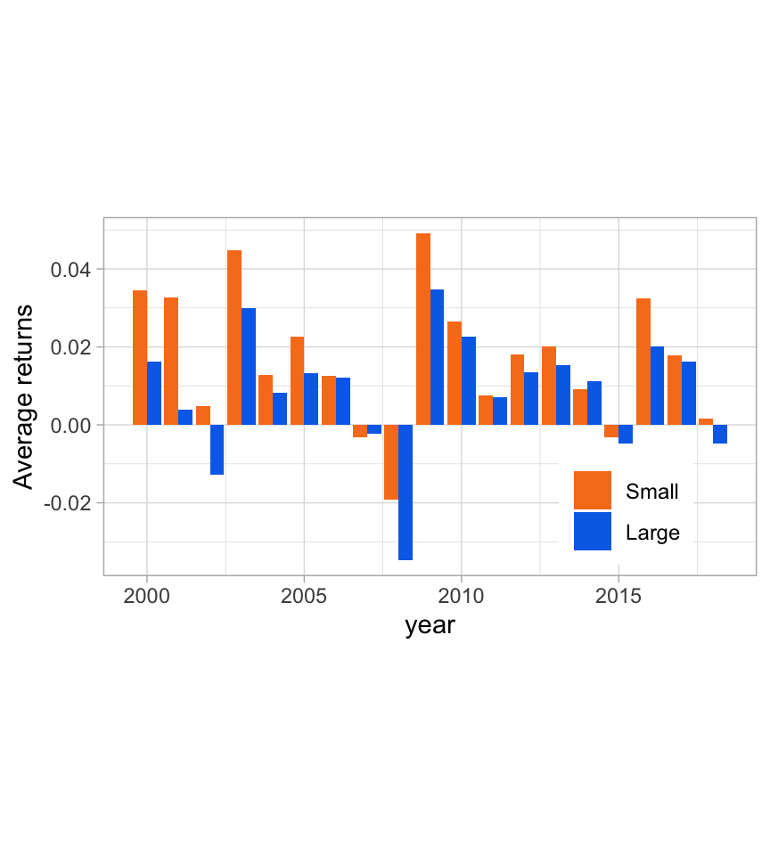
FIGURE 3.1: The size factor: average returns of small versus large firms.
3.2.3 Factors
The construction of so-called factors follows the same lines as above. Portfolios are based on one characteristic and the factor is a long-short ensemble of one extreme portfolio minus the opposite extreme (small minus large for the size factor or high book-to-market ratio minus low book-to-market ratio for the value factor). Sometimes, subtleties include forming bivariate sorts and aggregating several portfolios together, as in the original contribution of Fama and French (1993). The most common factors are listed below, along with a few references. We refer to the books listed at the beginning of the chapter for a more exhaustive treatment of factor idiosyncrasies. For most anomalies, theoretical justifications have been brought forward, whether risk-based or behavioral. We list the most frequently cited factors below:
- Size (SMB = small firms minus large firms): Banz (1981), Fama and French (1992), Fama and French (1993), Van Dijk (2011), Clifford Asness et al. (2018) and Astakhov, Havranek, and Novak (2019).
- Value (HML = high minus low: undervalued minus `growth’ firms): Fama and French (1992), Fama and French (1993), C. S. Asness, Moskowitz, and Pedersen (2013). See Israel, Laursen, and Richardson (2020) and Roca (2021) for recent discussions.
- Momentum (WML = winners minus losers): Jegadeesh and Titman (1993), Carhart (1997) and C. S. Asness, Moskowitz, and Pedersen (2013). The winners are the assets that have experienced the highest returns over the last year (sometimes the computation of the return is truncated to omit the last month). Cross-sectional momentum is linked, but not equivalent, to time series momentum (trend following), see e.g., Moskowitz, Ooi, and Pedersen (2012) and Lempérière et al. (2014). Momentum is also related to contrarian movements that occur both at higher and lower frequencies (short-term and long-term reversals), see Luo, Subrahmanyam, and Titman (2020).
- Profitability (RMW = robust minus weak profits): Fama and French (2015), Bouchaud et al. (2019). In the former reference, profitability is measured as (revenues - (cost and expenses))/equity.
- Investment (CMA = conservative minus aggressive): Fama and French (2015), Hou, Xue, and Zhang (2015). Investment is measured via the growth of total assets (divided by total assets). Aggressive firms are those that experience the largest growth in assets.
- Low `risk’ (sometimes, BAB = betting against beta): Ang et al. (2006), Baker, Bradley, and Wurgler (2011), Frazzini and Pedersen (2014), Boloorforoosh et al. (2020), Baker, Hoeyer, and Wurgler (2020) and Cliff Asness et al. (2020). In this case, the computation of risk changes from one article to the other (simple volatility, market beta, idiosyncratic volatility, etc.).
With the notable exception of the low risk premium, the most mainstream anomalies are kept and updated in the data library of Kenneth French (https://mba.tuck.dartmouth.edu/pages/faculty/ken.french/data_library.html). Of course, the computation of the factors follows a particular set of rules, but they are generally accepted in the academic sphere. Another source of data is the AQR repository: https://www.aqr.com/Insights/Datasets.
In the dataset we use for the book, we proxy the value anomaly not with the book-to-market ratio but with the price-to-book ratio (the book value is located in the denominator). As is shown in Clifford Asness and Frazzini (2013), the choice of the variable for value can have sizable effects.
Below, we import data from Ken French’s data library. A word of caution: the data is updated frequently and sometimes, experiences methodological changes. We refer to Akey, Robertson, and Simutin (2021) for a study of such changes in the common Fama-French factors. We will use this data later on in the chapter.
library(quantmod)                         # Package for data extraction
library(xtable)                           # Package for LaTeX exports
min_date <- "1963-07-31"                  # Start date
max_date <- "2020-03-28"                  # Stop date
temp <- tempfile()
KF_website <- "http://mba.tuck.dartmouth.edu/pages/faculty/ken.french/"
KF_file <- "ftp/F-F_Research_Data_5_Factors_2x3_CSV.zip"
link <- paste0(KF_website, KF_file)       # Link of the file
download.file(link, temp, quiet = TRUE)   # Download!
FF_factors <- read_csv(unz(temp, "F-F_Research_Data_5_Factors_2x3.csv"),
                       skip = 3) %>%          # Check the number of lines to skip!
    rename(date = `...1`, MKT_RF = `Mkt-RF`) %>%  # Change the name of first columns
    mutate_at(vars(-date), as.numeric) %>%                 # Convert values to number
    mutate(date = ymd(parse_date_time(date, "%Y%m"))) %>%  # Date in right format
    mutate(date = rollback(date + months(1)))              # End of month date
FF_factors <- FF_factors %>% mutate(MKT_RF = MKT_RF / 100, # Scale returns
                                    SMB = SMB / 100,
                                    HML = HML / 100,
                                    RMW = RMW / 100,
                                    CMA = CMA / 100,
                                    RF = RF/100) %>%
    filter(date >= min_date, date <= max_date)             # Finally, keep only recent points
knitr::kable(head(FF_factors),  booktabs = TRUE,
caption = "Sample of monthly factor returns.") # A look at the data (see table) | date | MKT_RF | SMB | HML | RMW | CMA | RF |
|---|---|---|---|---|---|---|
| 1963-07-31 | -0.0039 | -0.0041 | -0.0097 | 0.0068 | -0.0118 | 0.0027 |
| 1963-08-31 | 0.0507 | -0.0080 | 0.0180 | 0.0036 | -0.0035 | 0.0025 |
| 1963-09-30 | -0.0157 | -0.0052 | 0.0013 | -0.0071 | 0.0029 | 0.0027 |
| 1963-10-31 | 0.0253 | -0.0139 | -0.0010 | 0.0280 | -0.0201 | 0.0029 |
| 1963-11-30 | -0.0085 | -0.0088 | 0.0175 | -0.0051 | 0.0224 | 0.0027 |
| 1963-12-31 | 0.0183 | -0.0210 | -0.0002 | 0.0003 | -0.0007 | 0.0029 |
Posterior to the discovery of these stylized facts, some contributions have aimed at building theoretical models that capture these properties. We cite a handful below:
- size and value: Berk, Green, and Naik (1999), K. D. Daniel, Hirshleifer, and Subrahmanyam (2001), Barberis and Shleifer (2003), Gomes, Kogan, and Zhang (2003), Carlson, Fisher, and Giammarino (2004), R. D. Arnott et al. (2014);
- momentum: T. C. Johnson (2002), Grinblatt and Han (2005), Vayanos and Woolley (2013), Choi and Kim (2014).
In addition, recent bridges have been built between risk-based factor representations and behavioural theories. We refer essentially to Barberis, Mukherjee, and Wang (2016) and K. Daniel, Hirshleifer, and Sun (2020) and the references therein.
While these factors (i.e., long-short portfolios) exhibit time-varying risk premia and are magnified by corporate news and announcements (Engelberg, McLean, and Pontiff (2018)), it is well-documented (and accepted) that they deliver positive returns over long horizons.6 We refer to Gagliardini, Ossola, and Scaillet (2016) and to the survey Gagliardini, Ossola, and Scaillet (2019), as well as to the related bibliography for technical details on estimation procedures of risk premia and the corresponding empirical results. Large sample studies that documents regime changes in factor premia were also carried out by Ilmanen et al. (2019), S. Smith and Timmermann (2021) and Chib, Zhao, and Zhou (2021). Moreover, the predictability of returns is also time-varying (as documented in Farmer, Schmidt, and Timmermann (2019), Tsiakas, Li, and Zhang (2020) and Liu, Pan, and Wang (2020)), and estimation methods can be improved (T. L. Johnson (2019)).
In Figure 3.2, we plot the average monthly return aggregated over each calendar year for five common factors. The risk free rate (which is not a factor per se) is the most stable, while the market factor (aggregate market returns minus the risk-free rate) is the most volatile. This makes sense because it is the only long equity factor among the five series.
FF_factors %>%
    mutate(date = year(date)) %>%                       # Turn date into year
    gather(key = factor, value = value, - date) %>%     # Put in tidy shape
    group_by(date, factor) %>%                          # Group by year and factor
    summarise(value = mean(value)) %>%                  # Compute average return
    ggplot(aes(x = date, y = value, color = factor)) +  # Plot
    geom_line() + coord_fixed(500) + theme_light()      # Fix x/y ratio + theme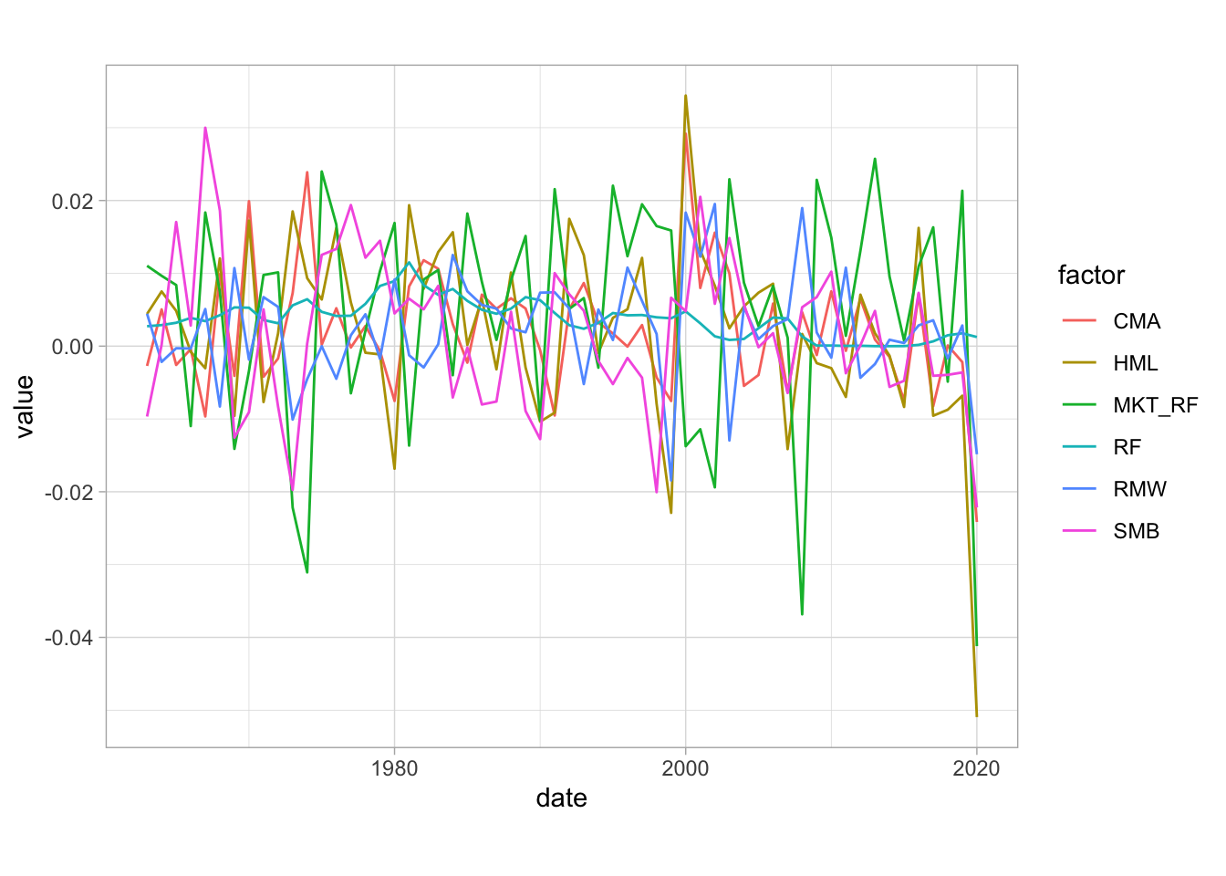
FIGURE 3.2: Average returns of common anomalies (1963-2020). Source: Ken French library.
The individual attributes of investors who allocate towards particular factors is a blossoming topic. We list a few references below, even though they somewhat lie out of the scope of this book. Betermier, Calvet, and Sodini (2017) show that value investors are older, wealthier and face lower income risk compared to growth investors who are those in the best position to take financial risks. The study Cronqvist, Siegel, and Yu (2015) leads to different conclusions: it finds that the propensity to invest in value versus growth assets has roots in genetics and in life events (the latter effect being confirmed in Cocco, Gomes, and Lopes (2020), and the former being further detailed in a more general context in Cronqvist et al. (2015)). Psychological traits can also explain some factors: when agents extrapolate, they are likely to fuel momentum (this topic is thoroughly reviewed in Barberis (2018)). Micro- and macro-economic consequences of these preferences are detailed in Bhamra and Uppal (2019). To conclude this paragraph, we mention that theoretical models have also been proposed that link agents’ preferences and beliefs (via prospect theory) to market anomalies (see for instance Barberis, Jin, and Wang (2020)).
Finally, we highlight the need of replicability of factor premia and echo the recent editorial by C. R. Harvey (2020). As is shown by Linnainmaa and Roberts (2018) and Hou, Xue, and Zhang (2020), many proclaimed factors are in fact very much data-dependent and often fail to deliver sustained profitability when the investment universe is altered or when the definition of variable changes (Clifford Asness and Frazzini (2013)).
Campbell Harvey and his co-authors, in a series of papers, tried to synthesize the research on factors in C. R. Harvey, Liu, and Zhu (2016), C. Harvey and Liu (2019) and C. R. Harvey and Liu (2019). His work underlines the need to set high bars for an anomaly to be called a ‘true’ factor. Increasing thresholds for \(p\)-values is only a partial answer, as it is always possible to resort to data snooping in order to find an optimized strategy that will fail out-of-sample but that will deliver a \(t\)-statistic larger than three (or even four). C. R. Harvey (2017) recommends to resort to a Bayesian approach which blends data-based significance with a prior into a so-called Bayesianized p-value (see subsection below).
Following this work, researchers have continued to explore the richness of this zoo. Bryzgalova, Huang, and Julliard (2019) propose a tractable Bayesian estimation of large-dimensional factor models and evaluate all possible combinations of more than 50 factors, yielding an incredibly large number of coefficients. This combined with a Bayesianized Fama and MacBeth (1973) procedure allows to distinguish between pervasive and superfluous factors. Chordia, Goyal, and Saretto (2020) use simulations of 2 million trading strategies to estimate the rate of false discoveries, that is, when a spurious factor is detected (type I error). They also advise to use thresholds for t-statistics that are well above three. In a similar vein, C. R. Harvey and Liu (2020) also underline that sometimes true anomalies may be missed because of a one time \(t\)-statistic that is too low (type II error).
The propensity of journals to publish positive results has led researchers to estimate the difference between reported returns and true returns. A. Y. Chen and Zimmermann (2020) call this difference the publication bias and estimate it as roughly 12%. That is, if a published average return is 8%, the actual value may in fact be closer to (1-12%)*8%=7%. Qualitatively, this estimation of 12% is smaller than the out-of-sample reduction in returns found in McLean and Pontiff (2016).
3.2.4 Predictive regressions, sorts, and p-value issues
For simplicity, we assume a simple form: \[\begin{equation} \tag{3.2} \textbf{r} = a+b\textbf{x}+\textbf{e}, \end{equation}\] where the vector \(\textbf{r}\) stacks all returns of all stocks and \(\textbf{x}\) is a lagged variable so that the regression is indeed predictive. If the estimate \(\hat{b}\) is significant given a specified threshold, then it can be tempting to conclude that \(\textbf{x}\) does a good job at predicting returns. Hence, long-short portfolios related to extreme values of \(\textbf{x}\) (mind the sign of \(\hat{b}\)) are expected to generate profits. This is unfortunately often false because \(\hat{b}\) gives information on the past ability of \(\textbf{x}\) to forecast returns. What happens in the future may be another story.
Statistical tests are also used for portfolio sorts. Assume two extreme portfolios are expected to yield very different average returns (like very small cap versus very large cap, or strong winners versus bad losers). The portfolio returns are written \(r_t^+\) and \(r_t^-\). The simplest test for the mean is \(t=\sqrt{T}\frac{m_{r_+}-m_{r_-}}{\sigma_{r_+-r_-}}\), where \(T\) is the number of points and \(m_{r_\pm}\) denotes the means of returns and \(\sigma_{r_+-r_-}\) is the standard deviation of the difference between the two series, i.e., the volatility of the long-short portfolio. In short, the statistic can be viewed as a scaled Sharpe ratio (though usually these ratios are computed for long-only portfolios) and can in turn be used to compute \(p\)-values to assess the robustness of an anomaly. As is shown in Linnainmaa and Roberts (2018) and Hou, Xue, and Zhang (2020), many factors discovered by researchers fail to survive in out-of-sample tests.
One reason why people are overly optimistic about anomalies they detect is the widespread reverse interpretation of the p-value. Often, it is thought of as the probability of one hypothesis (e.g., my anomaly exists) given the data. In fact, it’s the opposite; it’s the likelihood of your data sample, knowing that the anomaly holds. \[\begin{align*} p-\text{value} &= P[D|H] \\ \text{target prob.}& = P[H|D]=\frac{P[D|H]}{P[D]}\times P[H], \end{align*}\] where \(H\) stands for hypothesis and \(D\) for data. The equality in the second row is a plain application of Bayes’ identity: the interesting probability is in fact a transform of the \(p\)-value.
Two articles (at least) discuss this idea. C. R. Harvey (2017) introduces Bayesianized \(p\)-values: \[\begin{equation} \tag{3.3} \text{Bayesianized } p-\text{value}=\text{Bpv}= e^{-t^2/2}\times\frac{\text{prior}}{1+e^{-t^2/2}\times \text{prior}} , \end{equation}\] where \(t\) is the \(t\)-statistic obtained from the regression (i.e., the one that defines the p-value) and prior is the analyst’s estimation of the odds that the hypothesis (anomaly) is true. The prior is coded as follows. Suppose there is a p% chance that the null holds (i.e., (1-p)% for the anomaly). The odds are coded as \(p/(1-p)\). Thus, if the t-statistic is equal to 2 (corresponding to a p-value of 5% roughly) and the prior odds are equal to 6, then the Bpv is equal to \(e^{-2}\times 6 \times(1+e^{-2}\times 6)^{-1}\approx 0.448\) and there is a 44.8% chance that the null is true. This interpretation stands in sharp contrast with the original \(p\)-value which cannot be viewed as a probability that the null holds. Of course, one drawback is that the level of the prior is crucial and solely user-specified.
The work of Alexander Chinco, Neuhierl, and Weber (2020) is very different but shares some key concepts, like the introduction of Bayesian priors in regression outputs. They show that coercing the predictive regression with an \(L^2\) constraint (see the ridge regression in Chapter 5) amounts to introducing views on what the true distribution of \(b\) is. The stronger the constraint, the more the estimate \(\hat{b}\) will be shrunk towards zero. One key idea in their work is the assumption of a distribution for the true \(b\) across many anomalies. It is assumed to be Gaussian and centered. The interesting parameter is the standard deviation: the larger it is, the more frequently significant anomalies are discovered. Notably, the authors show that this parameter changes through time and we refer to the original paper for more details on this subject.
3.2.5 Fama-Macbeth regressions
Another detection method was proposed by Fama and MacBeth (1973) through a two-stage regression analysis of risk premia. The first stage is a simple estimation of the relationship (3.1): the regressions are run on a stock-by-stock basis over the corresponding time series. The resulting estimates \(\hat{\beta}_{i,k}\) are then plugged into a second series of regressions: \[\begin{equation} r_{t,n}= \gamma_{t,0} + \sum_{k=1}^K\gamma_{t,k}\hat{\beta}_{n,k} + \varepsilon_{t,n}, \end{equation}\] which are run date-by-date on the cross-section of assets.7 Theoretically, the betas would be known and the regression would be run on the \(\beta_{n,k}\) instead of their estimated values. The \(\hat{\gamma}_{t,k}\) estimate the premia of factor \(k\) at time \(t\). Under suitable distributional assumptions on the \(\varepsilon_{t,n}\), statistical tests can be performed to determine whether these premia are significant or not. Typically, the statistic on the time-aggregated (average) premia \(\hat{\gamma}_k=\frac{1}{T}\sum_{t=1}^T\hat{\gamma}_{t,k}\): \[t_k=\frac{\hat{\gamma}_k}{\hat{\sigma_k}/\sqrt{T}}\] is often used in pure Gaussian contexts to assess whether or not the factor is significant (\(\hat{\sigma}_k\) is the standard deviation of the \(\hat{\gamma}_{t,k}\)).
We refer to Jagannathan and Wang (1998) and Petersen (2009) for technical discussions on the biases and losses in accuracy that can be induced by standard ordinary least squares (OLS) estimations. Moreover, as the \(\hat{\beta}_{i,k}\) in the second-pass regression are estimates, a second level of errors can arise (the so-called errors in variables). The interested reader will find some extensions and solutions in Shanken (1992), Ang, Liu, and Schwarz (2018) and Jegadeesh et al. (2019).
Below, we perform Fama and MacBeth (1973) regressions on our sample. We start by the first pass: individual estimation of betas. We build a dedicated function below and use some functional programming to automate the process. We stick to the original implementation of the estimation and perform synchronous regressions.
nb_factors <- 5                                                     # Number of factors
data_FM <- left_join(data_ml %>%                                    # Join the 2 datasets
                         dplyr::select(date, stock_id, R1M_Usd) %>% # (with returns...
                         filter(stock_id %in% stock_ids_short),     # ... over some stocks)
                     FF_factors,
                     by = "date") %>%
    group_by(stock_id) %>%                                          # Grouping
    mutate(R1M_Usd = lag(R1M_Usd)) %>%                              # Lag returns
    ungroup() %>%
    na.omit() %>%                                                   # Remove missing points
    pivot_wider(names_from = "stock_id", values_from = "R1M_Usd")
models <- lapply(paste0("`", stock_ids_short,
                        '` ~  MKT_RF + SMB + HML + RMW + CMA'),           # Model spec
                 function(f){ lm(as.formula(f), data = data_FM,           # Call lm(.)
                                 na.action="na.exclude") %>%
                         summary() %>%                                    # Gather the output
                         "$"(coef) %>%                                    # Keep only coefs
                         data.frame() %>%                                 # Convert to dataframe
                         dplyr::select(Estimate)}                         # Keep the estimates
                 )
betas <- matrix(unlist(models), ncol = nb_factors + 1, byrow = T) %>%     # Extract the betas
    data.frame(row.names = stock_ids_short)                               # Format: row names
colnames(betas) <- c("Constant", "MKT_RF", "SMB", "HML", "RMW", "CMA") # Format: col names| Constant | MKT_RF | SMB | HML | RMW | CMA | |
|---|---|---|---|---|---|---|
| 1 | 0.008 | 1.417 | 0.529 | 0.621 | 0.980 | -0.379 |
| 3 | -0.002 | 0.812 | 1.108 | 0.882 | 0.300 | -0.552 |
| 4 | 0.004 | 0.363 | 0.306 | -0.050 | 0.595 | 0.200 |
| 7 | 0.005 | 0.431 | 0.675 | 0.230 | 0.322 | 0.177 |
| 9 | 0.004 | 0.838 | 0.678 | 1.057 | 0.078 | 0.062 |
| 11 | -0.001 | 0.986 | 0.121 | 0.483 | -0.124 | 0.018 |
In the table, MKT_RF is the market return minus the risk free rate. The corresponding coefficient is often referred to as the beta, especially in univariate regressions. We then reformat these betas from Table 3.2 to prepare the second pass. Each line corresponds to one asset: the first 5 columns are the estimated factor loadings and the remaining ones are the asset returns (date by date).
loadings <- betas %>%                            # Start from loadings (betas)
    dplyr::select(-Constant) %>%                 # Remove constant
    data.frame()                                 # Convert to dataframe
ret <- returns %>%                               # Start from returns
    dplyr::select(-date) %>%                     # Keep the returns only
    data.frame(row.names = returns$date) %>%     # Set row names
    t()                                          # Transpose
FM_data <- cbind(loadings, ret) # Aggregate both| MKT_RF | SMB | HML | RMW | CMA | 2000-01-31 | 2000-02-29 | 2000-03-31 | |
|---|---|---|---|---|---|---|---|---|
| 1 | 1.4173293 | 0.5292414 | 0.6206285 | 0.9800055 | -0.3788295 | -0.036 | 0.263 | 0.031 |
| 3 | 0.8120909 | 1.1083495 | 0.8824799 | 0.3002839 | -0.5520309 | 0.077 | -0.024 | 0.018 |
| 4 | 0.3629688 | 0.3061975 | -0.0504485 | 0.5954709 | 0.2003223 | -0.016 | 0.000 | 0.153 |
| 7 | 0.4314569 | 0.6748355 | 0.2303770 | 0.3220782 | 0.1773031 | -0.009 | 0.027 | 0.000 |
| 9 | 0.8381647 | 0.6775922 | 1.0571755 | 0.0777108 | 0.0622119 | 0.032 | 0.076 | -0.025 |
| 11 | 0.9858317 | 0.1205505 | 0.4833864 | -0.1244214 | 0.0175315 | 0.144 | 0.258 | 0.049 |
We observe that the values of the first column (market betas) revolve around one, which is what we would expect. Finally, we are ready for the second round of regressions.
models <- lapply(paste("`", returns$date, "`", ' ~  MKT_RF + SMB + HML + RMW + CMA', sep = ""),
function(f){ lm(as.formula(f), data = FM_data) %>%                        # Call lm(.)
                         summary() %>%                                    # Gather the output
                         "$"(coef) %>%                                    # Keep only the coefs
                         data.frame() %>%                                 # Convert to dataframe
                         dplyr::select(Estimate)}                         # Keep only estimates
                 )
gammas <- matrix(unlist(models), ncol = nb_factors + 1, byrow = T) %>%    # Switch to dataframe
    data.frame(row.names = returns$date)                                  # & set row names
colnames(gammas) <- c("Constant", "MKT_RF", "SMB", "HML", "RMW", "CMA") # Set col names| Constant | MKT_RF | SMB | HML | RMW | CMA | |
|---|---|---|---|---|---|---|
| 2000-01-31 | -0.011 | 0.041 | 0.223 | -0.143 | -0.276 | 0.033 |
| 2000-02-29 | 0.014 | 0.075 | -0.133 | 0.052 | 0.085 | -0.036 |
| 2000-03-31 | 0.004 | -0.010 | -0.013 | 0.049 | 0.040 | 0.050 |
| 2000-04-30 | 0.125 | -0.147 | -0.095 | 0.157 | 0.076 | -0.021 |
| 2000-05-31 | 0.052 | -0.011 | 0.074 | -0.096 | -0.095 | -0.056 |
| 2000-06-30 | 0.027 | -0.030 | -0.018 | 0.054 | 0.043 | 0.016 |
Visually, the estimated premia are also very volatile. We plot their estimated values for the market, SMB and HML factors.
gammas[2:nrow(gammas),] %>%                                         # Take gammas:
    # The first row is omitted because the first row of returns is undefined
    dplyr::select(MKT_RF, SMB, HML) %>%                             # Select 3 factors
    bind_cols(date = data_FM$date) %>%                              # Add date
    gather(key = factor, value = gamma, -date) %>%                  # Put in tidy shape
    ggplot(aes(x = date, y = gamma, color = factor)) +              # Plot
    geom_line() + facet_grid( factor~. ) +                          # Lines & facets
    scale_color_manual(values=c("#F87E1F", "#0570EA", "#F81F40")) + # Colors
    coord_fixed(980) + theme_light()                                # Fix x/y ratio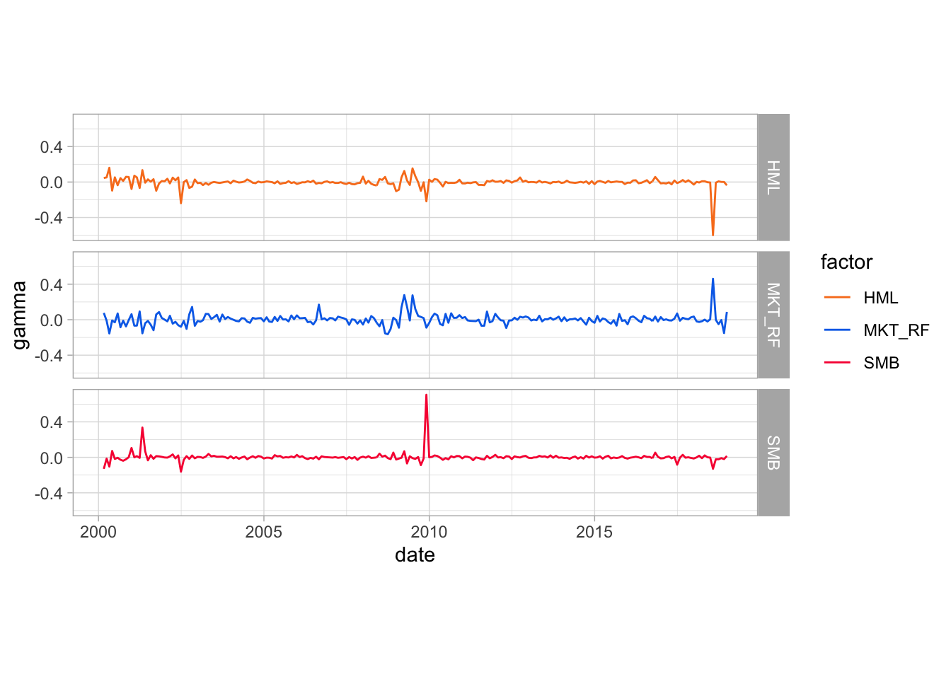
FIGURE 3.3: Time series plot of gammas (premia) in Fama-Macbeth regressions.
The two spikes at the end of the sample signal potential colinearity issues; two factors seem to compensate in an unclear aggregate effect. This underlines the usefulness of penalized estimates (see Chapter 5).
3.2.6 Factor competition
The core purpose of factors is to explain the cross-section of stock returns. For theoretical and practical reasons, it is preferable if redundancies within factors are avoided. Indeed, redundancies imply collinearity which is known to perturb estimates (Belsley, Kuh, and Welsch (2005)). In addition, when asset managers decompose the performance of their returns into factors, overlaps (high absolute correlations) between factors yield exposures that are less interpretable; positive and negative exposures compensate each other spuriously.
A simple protocol to sort out redundant factors is to run regressions of each factor against all others: \[\begin{equation} \tag{3.4} f_{t,k} = a_k +\sum_{j\neq k} \delta_{k,j} f_{t,j} + \epsilon_{t,k}. \end{equation}\] The interesting metric is then the test statistic associated to the estimation of \(a_k\). If \(a_k\) is significantly different from zero, then the cross-section of (other) factors fails to explain exhaustively the average return of factor \(k\). Otherwise, the return of the factor can be captured by exposures to the other factors and is thus redundant.
One mainstream application of this technique was performed in Fama and French (2015), in which the authors show that the HML factor is redundant when taking into account four other factors (Market, SMB, RMW and CMA). Below, we reproduce their analysis on an updated sample. We start our analysis directly with the database maintained by Kenneth French.
We can run the regressions that determine the redundancy of factors via the procedure defined in Equation (3.4).
factors <- c("MKT_RF", "SMB", "HML", "RMW", "CMA")
models <- lapply(paste(factors, ' ~  MKT_RF + SMB + HML + RMW + CMA-',factors),
 function(f){ lm(as.formula(f), data = FF_factors) %>%               # Call lm(.)
                         summary() %>%                               # Gather the output
                         "$"(coef) %>%                               # Keep only the coefs
                         data.frame() %>%                            # Convert to dataframe
                         filter(rownames(.) == "(Intercept)") %>%    # Keep only the Intercept
                         dplyr::select(Estimate,`Pr...t..`)}         # Keep the coef & p-value
                 )
alphas <- matrix(unlist(models), ncol = 2, byrow = T) %>%       # Switch from list to dataframe
    data.frame(row.names = factors)
# alphas # To see the alphas (optional)
We obtain the vector of \(\alpha\) values from Equation ((3.4)). Below, we format these figures along with \(p\)-value thresholds and export them in a summary table. The significance levels of coefficients is coded as follows: \(0<(***)<0.001<(**)<0.01<(*)<0.05\).
results <- matrix(NA, nrow = length(factors), ncol = length(factors) + 1)   # Coefs
signif  <- matrix(NA, nrow = length(factors), ncol = length(factors) + 1)   # p-values
for(j in 1:length(factors)){
    form <- paste(factors[j],
                  ' ~  MKT_RF + SMB + HML + RMW + CMA-',factors[j])         # Build model
    fit <- lm(form, data = FF_factors) %>% summary()                        # Estimate model
    coef <- fit$coefficients[,1]                                            # Keep coefficients
    p_val <- fit$coefficients[,4]                                           # Keep p-values
    results[j,-(j+1)] <- coef                                               # Fill matrix
    signif[j,-(j+1)] <- p_val
}
signif[is.na(signif)] <- 1                                                  # Kick out NAs
results <- results %>% round(3)  %>% data.frame()                           # Basic formatting
results[signif<0.001] <- paste(results[signif<0.001]," (***)")              # 3 star signif
results[signif>0.001&signif<0.01] <-                                        # 2 star signif
    paste(results[signif>0.001&signif<0.01]," (**)")
results[signif>0.01&signif<0.05] <-                                         # 1 star signif
    paste(results[signif>0.01&signif<0.05]," (*)")
results <- cbind(as.character(factors), results)                            # Add dep. variable
colnames(results) <- c("Dep. Variable","Intercept", factors)                # Add column names
| Dep. Variable | Intercept | MKT_RF | SMB | HML | RMW | CMA |
|---|---|---|---|---|---|---|
| MKT_RF | 0.008 (***) | NA | 0.257 (***) | 0.12 | -0.363 (***) | -0.945 (***) |
| SMB | 0.003 (*) | 0.131 (***) | NA | 0.083 | -0.435 (***) | -0.139 |
| HML | -0.001 | 0.032 | 0.044 | NA | 0.169 (***) | 1.027 (***) |
| RMW | 0.004 (***) | -0.096 (***) | -0.225 (***) | 0.165 (***) | NA | -0.319 (***) |
| CMA | 0.002 (***) | -0.112 (***) | -0.032 | 0.45 (***) | -0.144 (***) | NA |
We confirm that the HML factor remains redundant when the four others are present in the asset pricing model. The figures we obtain are very close to the ones in the original paper (Fama and French (2015)), which makes sense, since we only add 5 years to their initial sample.
At a more macro-level, researchers also try to figure out which models (i.e., combinations of factors) are the most likely, given the data empirically observed (and possibly given priors formulated by the econometrician). For instance, this stream of literature seeks to quantify to which extent the 3-factor model of Fama and French (1993) outperforms the 5 factors in Fama and French (2015). In this direction, De Moor, Dhaene, and Sercu (2015) introduce a novel computation for p-values that compare the relative likelihood that two models pass a zero-alpha test. More generally, the Bayesian method of Barillas and Shanken (2018) was subsequently improved by Chib, Zeng, and Zhao (2020) - see also Chib and Zeng (2020) and Chib et al. (2020) (an R package exists for the former: czfactor). For a discussion on model comparison from a transaction cost perspective, we refer to S. A. Li, DeMiguel, and Martin-Utrera (2020).
Lastly, even the optimal number of factors is a subject of disagreement among conclusions of recent work. While the traditional literature focuses on a limited number (3-5) of factors (see also Hwang and Rubesam (2021)), more recent research by DeMiguel et al. (2020), A. He, Huang, and Zhou (2020), Kozak, Nagel, and Santosh (2019) and Freyberger, Neuhierl, and Weber (2020) advocates the need to use at least 15 or more (in contrast, Kelly, Pruitt, and Su (2019) argue that a small number of latent factors may suffice). Green, Hand, and Zhang (2017) even find that the number of characteristics that help explain the cross-section of returns varies in time.8
3.2.7 Advanced techniques
The ever increasing number of factors combined to their importance in asset management has led researchers to craft more subtle methods in order to ``organize’’ the so-called factor zoo and, more importantly, to detect spurious anomalies and compare different asset pricing model specifications. We list a few of them below.
- Feng, Giglio, and Xiu (2020) combine LASSO selection with Fama-MacBeth regressions to test if new factor models are worth it. They quantify the gain of adding one new factor to a set of predefined factors and show that many factors reported in papers published in the 2010 decade do not add much incremental value;
- C. Harvey and Liu (2019) (in a similar vein) use bootstrap on orthogonalized factors. They make the case that correlations among predictors is a major issue and their method aims at solving this problem. Their lengthy procedure seeks to test if maximal additional contribution of a candidate variable is significant;
- Fama and French (2018) compare asset pricing models through squared maximum Sharpe ratios;
- Giglio and Xiu (2019) estimate factor risk premia using a three-pass method based on principal component analysis;
- Pukthuanthong, Roll, and Subrahmanyam (2018) disentangle priced and non-priced factors via a combination of principal component analysis and Fama and MacBeth (1973) regressions;
- Gospodinov, Kan, and Robotti (2019) warn against factor misspecification (when spurious factors are included in the list of regressors). Traded factors (\(resp.\) macro-economic factors) seem more likely (\(resp.\) less likely) to yield robust identifications (see also Bryzgalova (2019)).
There is obviously no infallible method, but the number of contributions in the field highlights the need for robustness. This is evidently a major concern when crafting investment decisions based on factor intuitions. One major hurdle for short-term strategies is the likely time-varying feature of factors. We refer for instance to Ang and Kristensen (2012), Cooper and Maio (2019), and Briere and Szafarz (2021) for practical results and to Gagliardini, Ossola, and Scaillet (2016) and S. Ma et al. (2020) for more theoretical treatments (with additional empirical results).
3.3 Factors or characteristics?
The decomposition of returns into linear factor models is convenient because of its simple interpretation. There is nonetheless a debate in the academic literature about whether firm returns are indeed explained by exposure to macro-economic factors or simply by the characteristics of firms. In their early study, Lakonishok, Shleifer, and Vishny (1994) argue that one explanation of the value premium comes from incorrect extrapolation of past earning growth rates. Investors are overly optimistic about firms subject to recent profitability. Consequently, future returns are (also) driven by the core (accounting) features of the firm. The question is then to disentangle which effect is the most pronounced when explaining returns: characteristics versus exposures to macro-economic factors.
In their seminal contribution on this topic, K. Daniel and Titman (1997) provide evidence in favour of the former (two follow-up papers are K. Daniel, Titman, and Wei (2001) and K. Daniel and Titman (2012)). They show that firms with high book-to-market ratios or small capitalizations display higher average returns, even if they are negatively loaded on the HML or SMB factors. Therefore, it seems that it is indeed the intrinsic characteristics that matter, and not the factor exposure. For further material on characteristics’ role in return explanation or prediction, we refer to the following contributions:
- Haugen and Baker (1996) estimate predictive regressions based on firms characteristics and show that it is possible to build profitable portfolios based on the resulting predictions. There method was subsequently enhanced with the adaptive LASSO by Guo (2020).
- Section 2.5.2. in Goyal (2012) surveys pre-2010 results on this topic;
- Chordia, Goyal, and Shanken (2019) find that characteristics explain a larger proportion of variation in estimated expected returns than factor loadings;
- Kozak, Nagel, and Santosh (2018) reconcile factor-based explanations of premia to a theoretical model in which some agents’ demands are sentiment driven;
- Han et al. (2019) show with penalized regressions that 20 to 30 characteristics (out of 94) are useful for the prediction of monthly returns of US stocks. Their methodology is interesting: they regress returns against characteristics to build forecasts and then regress the returns on the forecast to assess if they are reliable. The latter regression uses a LASSO-type penalization (see Chapter 5) so that useless characteristics are excluded from the model. The penalization is extended to elasticnet in D. Rapach and Zhou (2019).
- Kelly, Pruitt, and Su (2019) and S. Kim, Korajczyk, and Neuhierl (2019) both estimate models in which factors are latent but loadings (betas) and possibly alphas depend on characteristics. Kirby (2020) generalizes the first approach by introducing regime-switching. In contrast, Lettau and Pelger (2020a) and Lettau and Pelger (2020b) estimate latent factors without any link to particular characteristics (and provide large sample asymptotic properties of their methods).
- In the same vein as Hoechle, Schmid, and Zimmermann (2018), Gospodinov, Kan, and Robotti (2019) and Bryzgalova (2019) and discuss potential errors that arise when working with portfolio sorts that yield long-short returns. The authors show that in some cases, tests based on this procedure may be deceitful. This happens when the characteristic chosen to perform the sort is correlated with an external (unobservable) factor. They propose a novel regression-based approach aimed at bypassing this problem.
More recently and in a separate stream of literature, R. S. J. Koijen and Yogo (2019) have introduced a demand model in which investors form their portfolios according to their preferences towards particular firm characteristics. They show that this allows them to mimic the portfolios of large institutional investors. In their model, aggregate demands (and hence, prices) are directly linked to characteristics, not to factors. In a follow-up paper, R. S. Koijen, Richmond, and Yogo (2019) show that a few sets of characteristics suffice to predict future returns. They also show that, based on institutional holdings from the UK and the US, the largest investors are those who are the most influencial in the formation of prices. In a similar vein, Betermier, Calvet, and Jo (2019) derive an elegant (theoretical) general equilibrium model that generates some well-documented anomalies (size, book-to-market). The models of R. D. Arnott et al. (2014) and Alti and Titman (2019) are also able to theoretically generate known anomalies. Finally, in I. Martin and Nagel (2019), characteristics influence returns via the role they play in the predictability of dividend growth. This paper discussed the asymptotic case when the number of assets and the number of characteristics are proportional and both increase to infinity.
3.4 Hot topics: momentum, timing and ESG
3.4.1 Factor momentum
A recent body of literature unveils a time series momentum property of factor returns. For instance, T. Gupta and Kelly (2019) report that autocorrelation patterns within these returns is statistically significant.9 Similar results are obtained in Falck, Rej, and Thesmar (2022). In the same vein, R. D. Arnott et al. (2021) make the case that the industry momentum found in Moskowitz and Grinblatt (1999) can in fact be explained by this factor momentum. Going even further, Ehsani and Linnainmaa (2022) conclude that the original momentum factor is in fact the aggregation of the autocorrelation that can be found in all other factors. Recently, the strength of factor momentum is scrutinized by Fan et al. (2021). The authors find that it is only robust for a small number of factors.
Acknowledging the profitability of factor momentum, H. Yang (2020b) seeks to understand its source and decomposes stock factor momentum portfolios into two components: factor timing portfolio and a static portfolio. The former seeks to profit from the serial correlations of factor returns while the latter tries to harness factor premia. The author shows that it is the static portfolio that explains the larger portion of factor momentum returns. In H. Yang (2020a), the same author presents a new estimator to gauge factor momentum predictability. Words of caution are provided in Leippold and Yang (2021).
Lastly, Garcia, Medeiros, and Ribeiro (2021) document factor momentum at the daily frequency.
Given the data obtained on Ken French’s website, we compute the autocorrelation function (ACF) of factors. We recall that \[\text{ACF}_k(\textbf{x}_t)=\mathbb{E}[(\textbf{x}_t-\bar{\textbf{x}})(\textbf{x}_{t+k}-\bar{\textbf{x}})].\]
library(cowplot)                   # For stacking plots
library(forecast)                  # For autocorrelation function
acf_SMB <- ggAcf(FF_factors$SMB, lag.max = 10) + labs(title = "")  # ACF SMB
acf_HML <- ggAcf(FF_factors$HML, lag.max = 10) + labs(title = "")  # ACF HML
acf_RMW <- ggAcf(FF_factors$RMW, lag.max = 10) + labs(title = "")  # ACF RMW
acf_CMA <- ggAcf(FF_factors$CMA, lag.max = 10) + labs(title = "")  # ACF CMA
plot_grid(acf_SMB, acf_HML, acf_RMW, acf_CMA,  # Plot
labels = c('SMB', 'HML', 'RMW', 'CMA')) 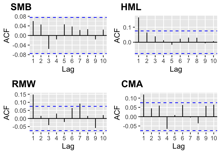
FIGURE 3.4: Autocorrelograms of common factor portfolios.
Of the four chosen series, only the size factor is not significantly autocorrelated at the first order.
3.4.2 Factor timing
Given the abundance of evidence of the time-varying nature of factor premia, it is legitimate to wonder if it is possible to predict when factor will perform well or badly. The evidence on the effectiveness of timing is diverse: positive for Greenwood and Hanson (2012), Hodges et al. (2017), Hasler, Khapko, and Marfe (2019), Haddad, Kozak, and Santosh (2020), Lioui and Tarelli (2020) and Neuhierl et al. (2023) more recently, but negative for Clifford Asness et al. (2017) and mixed for Dichtl et al. (2019). The majority of positive findings may be due to the bias towards positive results - but this is pure speculation.
There is no consensus on which predictors to use (general macroeconomic indicators in Hodges et al. (2017), stock issuances versus repurchases in Greenwood and Hanson (2012), and aggregate fundamental data in Dichtl et al. (2019)). A method for building reasonable timing strategies for long-only portfolios with sustainable transaction costs is laid out in Leippold and Rüegg (2020). The cross-section of characteristics is used for factor timing purposes in Kagkadis et al. (2021). In Vincenz and Zeissler (2021), it is found that macro variables are the best for this purpose. In ML-based factor investing, it is possible to resort to more granularity by combining firm-specific attributes to large-scale economic data as we explain in Section 4.7.2.
3.4.3 The green factors
The demand for ethical financial products has sharply risen during the 2010 decade, leading to the creation of funds dedicated to socially responsible investing (SRI - see Camilleri (2020)). Though this phenomenon is not really new (Schueth (2003), Hill et al. (2007)), its acceleration has prompted research about whether or not characteristics related to ESG criteria (environment, social, governance) are priced. Dozens and even possibly hundreds of papers have been devoted to this question, but no consensus has been reached. More and more, researchers study the financial impact of climate change (see Bernstein, Gustafson, and Lewis (2019), Hong, Li, and Xu (2019) and Hong, Karolyi, and Scheinkman (2020)) and the societal push for responsible corporate behavior (Fabozzi (2020), Kurtz (2020)). We gather below a very short list of papers that suggests conflicting results:
-
favorable: ESG investing works (Kempf and Osthoff (2007), Cheema-Fox et al. (2020)), can work (Nagy, Kassam, and Lee (2016), Alessandrini and Jondeau (2020)), or can at least be rendered efficient (Branch and Cai (2012)). A large meta-study reports overwhelming favorable results (Friede, Busch, and Bassen (2015)), but of course, they could well stem from the publication bias towards positive results.
-
unfavorable: Ethical investing is not profitable according to Adler and Kritzman (2008) and Blitz and Swinkels (2020). An ESG factor should be long unethical firms and short ethical ones (Lioui (2018)).
- mixed: ESG investing may be beneficial globally but not locally (Chakrabarti and Sen (2020)). Portfolios relying on ESG screening do not significantly outperform those with no screening but are subject to lower levels of volatility (Gibson et al. (2020), Gougler and Utz (2020)). As is often the case, the devil is in the details, and results depend on whether to use E, S or G (Bruder et al. (2019)).
On top of these contradicting results, several articles point towards complexities in the measurement of ESG. Depending on the chosen criteria and on the data provider, results can change drastically (see Galema, Plantinga, and Scholtens (2008), Berg, Koelbel, and Rigobon (2020) and Atta-Darkua et al. (2020)).
We end this short section by noting that of course ESG criteria can directly be integrated into ML model, as is for instance done in Franco et al. (2020).
3.5 The links with machine learning
Given the exponential increase in data availability, the obvious temptation of any asset manager is to try to infer future returns from the abundance of attributes available at the firm level. We allude to classical data like accounting ratios and to alternative data, such as sentiment. This task is precisely the aim of Machine Learning. Given a large set of predictor variables (\(\mathbf{X}\)), the goal is to predict a proxy for future performance \(\mathbf{y}\) through a model of the form (2.1).
If fundamental data (accounting ratios, earnings, relative valuations, etc.) help predict returns, then one refinement is to predict this fundamental data upfront. This may allow to anticipate changes or gain informational edges. Recent contributions in this directions include K. Cao and You (2020) and D. Huang et al. (2020).
Some earlier attempts have already been made that aim to explain and predict returns with firm attributes (e.g., Brandt, Santa-Clara, and Valkanov (2009), Hjalmarsson and Manchev (2012), Ammann, Coqueret, and Schade (2016), DeMiguel et al. (2020) and McGee and Olmo (2020)), but not with any ML intent or focus originally. In retrospect, these approaches do share some links with ML tools. The general formulation is the following. At time \(T\), the agent or investor seeks to solve the following program: \[\begin{align*} \underset{\boldsymbol{\theta}_T}{\max} \ \mathbb{E}_T\left[ u(r_{p,T+1})\right] = \underset{\boldsymbol{\theta}_T}{\max} \ \mathbb{E}_T\left[ u\left(\left(\bar{\textbf{w}}_T+\textbf{x}_T\boldsymbol{\theta}_T\right)'\textbf{r}_{T+1}\right)\right] , \end{align*}\] where \(u\) is some utility function and \(r_{p,T+1}=\left(\bar{\textbf{w}}_T+\textbf{x}_T\boldsymbol{\theta}_T\right)'\textbf{r}_{T+1}\) is the return of the portfolio, which is defined as a benchmark \(\bar{\textbf{w}}_T\) plus some deviations from this benchmark that are a linear function of features \(\textbf{x}_T\boldsymbol{\theta}_T\). The above program may be subject to some external constraints (e.g., to limit leverage).
In practice, the vector \(\boldsymbol{\theta}_T\) must be estimated using past data (from \(T-\tau\) to \(T-1\)): the agent seeks the solution of \[\begin{align} \tag{3.5} \underset{\boldsymbol{\theta}_T}{\text{max}} \ \frac{1}{\tau} \sum_{t=T-\tau}^{T-1} u \left( \sum_{i=1}^{N_T}\left(\bar{w}_{i,t}+ \boldsymbol{\theta}'_T \textbf{x}_{i,t} \right)r_{i,t+1} \right) \end{align}\]
on a sample of size \(\tau\) where \(N_T\) is the number of asset in the universe. The above formulation can be viewed as a learning task in which the parameters are chosen such that the reward (average return) is maximized.
3.5.1 A short list of recent references
Independent of a characteristics-based approach, ML applications in finance have blossomed, initially working with price data only and later on integrating firm characteristics as predictors. We cite a few references below, grouped by methodological approach:
- penalized quadratic programming: Goto and Xu (2015), Ban, El Karoui, and Lim (2016) and Perrin and Roncalli (2019),
- regularized predictive regressions: D. E. Rapach, Strauss, and Zhou (2013) and Alexander Chinco, Clark-Joseph, and Ye (2019),
- support vector machines: L.-J. Cao and Tay (2003) (and the references therein),
- model comparison and/or aggregation: K. Kim (2003), W. Huang, Nakamori, and Wang (2005), Matı́as and Reboredo (2012), Reboredo, Matı́as, and Garcia-Rubio (2012), Dunis et al. (2013), Gu, Kelly, and Xiu (2020b), Guida and Coqueret (2018b) and Tobek and Hronec (2021). The latter two more recent articles work with a large cross-section of characteristics.
We provide more detailed lists for tree-based methods, neural networks and reinforcement learning techniques in Chapters 6, 7 and 16, respectively. Moreover, we refer to Ballings et al. (2015) for a comparison of classifiers and to Henrique, Sobreiro, and Kimura (2019) and Bustos and Pomares-Quimbaya (2020) for surveys on ML-based forecasting techniques.
3.5.2 Explicit connections with asset pricing models
The first and obvious link between factor investing and asset pricing is (average) return prediction. The main canonical academic reference is Gu, Kelly, and Xiu (2020b). Let us first write the general equation and then comment on it: \[\begin{equation} \tag{3.6} r_{t+1,n}=g(\textbf{x}_{t,n}) + \epsilon_{t+1}. \end{equation}\]
The interesting discussion lies in the differences between the above model and that of Equation (3.1). The first obvious difference is the introduction of the nonlinear function \(g\): indeed, there is no reason (beyond simplicity and interpretability) why we should restrict the model to linear relationships. One early reference for nonlinearities in asset pricing kernels is Bansal and Viswanathan (1993).
More importantly, the second difference between (3.6) and (3.1) is the shift in the time index. Indeed, from an investor’s perspective, the interest is to be able to predict some information about the structure of the cross-section of assets. Explaining asset returns with synchronous factors is not useful because the realization of factor values is not known in advance. Hence, if one seeks to extract value from the model, there needs to be a time interval between the observation of the state space (which we call \(\textbf{x}_{t,n}\)) and the occurrence of the returns. Once the model \(\hat{g}\) is estimated, the time-\(t\) (measurable) value \(g(\textbf{x}_{t,n})\) will give a forecast for the (average) future returns. These predictions can then serve as signals in the crafting of portfolio weights (see Chapter 12 for more on that topic).
While most studies do work with returns on the l.h.s. of (3.6), there is no reason why other indicators should not be used. Returns are straightforward and simple to compute, but they could very well be replaced by more sophisticated metrics, like the Sharpe ratio, for instance. The firms’ features would then be used to predict a risk-adjusted performance rather than simple returns.
Beyond the explicit form of Equation (3.6), several other ML-related tools can also be used to estimate asset pricing models. This can be achieved in several ways, some of which we list below.
First, one mainstream problem in asset pricing is to characterize the stochastic discount factor (SDF) \(M_t\), which satisfies \(\mathbb{E}_t[M_{t+1}(r_{t+1,n}-r_{t+1,f})]=0\) for any asset \(n\) (see Cochrane (2009)). This equation is a natural playing field for the generalized method of moment (Hansen (1982)): \(M_t\) must be such that \[\begin{equation} \tag{3.7} \mathbb{E}[M_{t+1}R_{t+1,n}g(V_t)]=0, \end{equation}\] where the instrumental variables \(V_t\) are \(\mathcal{F}_t\)-measurable (i.e., are known at time \(t\)) and the capital \(R_{t+1,n}\) denotes the excess return of asset \(n\). In order to reduce and simplify the estimation problem, it is customary to define the SDF as a portfolio of assets (see chapter 3 in Back (2010)). In Luyang Chen, Pelger, and Zhu (2020), the authors use a generative adversarial network (GAN, see Section 7.7.1) to estimate the weights of the portfolios that are the closest to satisfy (3.7) under a strongly penalizing form.
A second approach is to try to model asset returns as linear combinations of factors, just as in (3.1). We write in compact notation \[r_{t,n}=\alpha_n+\boldsymbol{\beta}_{t,n}'\textbf{f}_t+\epsilon_{t,n},\] and we allow the loadings \(\boldsymbol{\beta}_{t,n}\) to be time-dependent. The trick is then to introduce the firm characteristics in the above equation. Traditionally, the characteristics are present in the definition of factors (as in the seminal definition of Fama and French (1993)). The decomposition of the return is made according to the exposition of the firm’s return to these factors constructed according to market size, accounting ratios, past performance, etc. Given the exposures, the performance of the stock is attributed to particular style profiles (e.g., small stock, or value stock, etc.).
Habitually, the factors are heuristic portfolios constructed from simple rules like thresholding. For instance, firms below the 1/3 quantile in book-to-market are growth firms and those above the 2/3 quantile are the value firms. A value factor can then be defined by the long-short portfolio of these two sets, with uniform weights. Note that Fama and French (1993) use a more complex approach which also takes market capitalization into account both in the weighting scheme and also in the composition of the portfolios.
One of the advances enabled by machine learning is to automate the construction of the factors. It is for instance the approach of Feng, Polson, and Xu (2019). Instead of building the factors heuristically, the authors optimize the construction to maximize the fit in the cross-section of returns. The optimization is performed via a relatively deep feed-forward neural network and the feature space is lagged so that the relationship is indeed predictive, as in Equation (3.6). Theoretically, the resulting factors help explain a substantially larger proportion of the in-sample variance in the returns. The prediction ability of the model depends on how well it generalizes out-of-sample.
A third approach is that of Kelly, Pruitt, and Su (2019) (though the statistical treatment is not machine learning per se).10 Their idea is the opposite: factors are latent (unobserved) and it is the betas (loadings) that depend on the characteristics. This allows many degrees of freedom because in \(r_{t,n}=\alpha_n+(\boldsymbol{\beta}_{t,n}(\textbf{x}_{t-1,n}))'\textbf{f}_t+\epsilon_{t,n},\) only the characteristics \(\textbf{x}_{t-1,n}\) are known and both the factors \(\textbf{f}_t\) and the functional forms \(\boldsymbol{\beta}_{t,n}(\cdot)\) must be estimated. In their article, Kelly, Pruitt, and Su (2019) work with a linear form, which is naturally more tractable.
Lastly, a fourth approach (introduced in Gu, Kelly, and Xiu (2020a)) goes even further and combines two neural network architectures. The first neural network takes characteristics \(\textbf{x}_{t-1}\) as inputs and generates factor loadings \(\boldsymbol{\beta}_{t-1}(\textbf{x}_{t-1})\). The second network transforms returns \(\textbf{r}_t\) into factor values \(\textbf{f}_t(\textbf{r}_t)\) (in Feng, Polson, and Xu (2019)). The aggregate model can then be written: \[\begin{equation} \tag{3.8} \textbf{r}_t=\boldsymbol{\beta}_{t-1}(\textbf{x}_{t-1})'\textbf{f}_t(\textbf{r}_t)+\boldsymbol{\epsilon}_t. \end{equation}\]
The above specification is quite special because the output (on the l.h.s.) is also present as input (in the r.h.s.). In machine learning, autoencoders (see Section 7.7.2) share the same property. Their aim, just like in principal component analysis, is to find a parsimonious nonlinear representation form for a dataset (in this case, returns). In Equation (3.8), the input is \(\textbf{r}_t\) and the output function is \(\boldsymbol{\beta}_{t-1}(\textbf{x}_{t-1})'\textbf{f}_t(\textbf{r}_t)\). The aim is to minimize the difference between the two just as is any regression-like model.
Autoencoders are neural networks which have outputs as close as possible to the inputs with an objective of dimensional reduction. The innovation in Gu, Kelly, and Xiu (2020a) is that the pure autoencoder part is merged with a vanilla perceptron used to model the loadings. The structure of the neural network is summarized below.
\[\left. \begin{array}{rl} \text{returns } (\textbf{r}_t) & \overset{NN_1}{\longrightarrow} \quad \text{ factors } (\textbf{f}_t=NN_1(\textbf{r}_t)) \\ \text{characteristics } (\textbf{x}_{t-1}) & \overset{NN_2}{\longrightarrow} \quad \text{ loadings } (\boldsymbol{\beta}_{t-1}=NN_2(\textbf{x}_{t-1})) \end{array} \right\} \longrightarrow \text{ returns } (r_t)\]
A simple autoencoder would consist of only the first line of the model. This specification is discussed in more details in Section 7.7.2.
As a conclusion of this chapter, it appears undeniable that the intersection between the two fields of asset pricing and machine learning offers a rich variety of applications. The literature is already exhaustive and it is often hard to disentangle the noise from the great ideas in the continuous flow of publications on these topics. Practice and implementation is the only way forward to extricate value from hype. This is especially true because agents often tend to overestimate the role of factors in the allocation decision process of real-world investors (see Alex Chinco, Hartzmark, and Sussman (2019) and Castaneda and Sabat (2019)).
3.6 Coding exercises
- Compute annual returns of the growth versus value portfolios, that is, the average return of firms with above median price-to-book ratio (the variable is called `Pb’ in the dataset).
- Same exercise, but compute the monthly returns and plot the value (through time) of the corresponding portfolios.
- Instead of a unique threshold, compute simply sorted portfolios based on quartiles of market capitalization. Compute their annual returns and plot them.