7 Neural networks

Neural networks (NNs) are an immensely rich and complicated topic. In this chapter, we introduce the simple ideas and concepts behind the most simple architectures of NNs. For more exhaustive treatments on NN idiosyncracies, we refer to the monographs by Haykin (2009), K.-L. Du and Swamy (2013) and Goodfellow et al. (2016). The latter is available freely online: www.deeplearningbook.org. For a practical introduction, we recommend the great book of Chollet (2017).

For starters, we briefly comment on the qualification “neural network”. Most experts agree that the term is not very well chosen, as NNs have little to do with how the human brain works (of which we know not that much). This explains why they are often referred to as “artificial neural networks” - we do not use the adjective for notational simplicity. Because we consider it more appropriate, we recall the definition of NNs given by François Chollet: “chains of differentiable, parameterised geometric functions, trained with gradient descent (with gradients obtained via the chain rule)”.

Early references of neural networks in finance are Bansal and Viswanathan (1993) and Eakins, Stansell, and Buck (1998). Both have very different goals. In the first one, the authors aim to estimate a nonlinear form for the pricing kernel. In the second one, the purpose is to identify and quantify relationships between institutional investments in stocks and the attributes of the firms (an early contribution towards factor investing). An early review (Burrell and Folarin (1997)) lists financial applications of NNs during the 1990s. More recently, Sezer, Gudelek, and Ozbayoglu (2019), W. Jiang (2020) and Lim and Zohren (2021) survey the attempts to forecast financial time series with deep-learning models, mainly by computer science scholars.

The pure predictive ability of NNs in financial markets is a popular subject and we further cite for example Kimoto et al. (1990), Enke and Thawornwong (2005), Y. Zhang and Wu (2009), Guresen, Kayakutlu, and Daim (2011), Krauss, Do, and Huck (2017), Fischer and Krauss (2018), Aldridge and Avellaneda (2019), Babiak and Barunik (2020), Y. Ma, Han, and Wang (2020), and Soleymani and Paquet (2020).^[Neural networks have also been recently applied to derivatives pricing and hedging, see for instance the work of Buehler et al. (2019) and Andersson and Oosterlee (2020) and the survey by Ruf and Wang (2019). In Wu et al. (2020), it is found that deep learning is efficient for selecting performing hedge funds. Some article find that NNs underperform in the task of stock market prediction (and on tabular data more generally). Y. Wei (2021) argues that it is because RMSE is not suited for stock return forecasts for which it is the direction that matters (though of course, the direction could also be the label!).

Limit order book modelling is also an expanding field for neural network applications (Sirignano and Cont (2019), Wallbridge (2020)).] The last reference even combines several types of NNs embedded inside an overarching reinforcement learning structure. This list is very far from exhaustive. In the field of financial economics, recent research on neural networks includes:

• Feng, Polson, and Xu (2019) use neural networks to find factors that are the best at explaining the cross-section of stock returns.
  
• Gu, Kelly, and Xiu (2020b) map firm attributes and macro-economic variables into future returns. This creates a strong predictive tool that is able to forecast future returns very accurately.
  
• Luyang Chen, Pelger, and Zhu (2020) estimate the pricing kernel with a complex neural network structure including a generative adversarial network. This again gives crucial information on the structure of expected stock returns and can be used for portfolio construction (by building an accurate maximum Sharpe ratio policy).

7.1 The original perceptron

The origins of NNs go back at least to Rosenblatt (1958). Its aim is binary classification. For simplicity, let us assume that the output is \(\{0\) = do not invest\(\}\) versus \(\{1\) = invest\(\}\) (e.g., derived from return, negative versus positive). Given the current nomenclature, a perceptron can be defined as an activated linear mapping. The model is the following:

\[f(\mathbf{x})=\left\{ \begin{array}{lll} 1 & \text{if } \mathbf{x}'\mathbf{w}+b >0\\ 0 &\text{otherwise} \end{array}\right.\] The vector of weights \(\mathbf{w}\) scales the variables and the bias \(b\) shifts the decision barrier. Given values for \(b\) and \(w_i\), the error is \(\epsilon_i=y_i-1_{\left\{\sum_{j=1}^Jx_{i,j}w_j+w_0>0\right\}}\). As is customary, we set \(b=w_0\) and add an initial constant column to \(x\): \(x_{i,0}=1\), so that \(\epsilon_i=y_i-1_{\left\{\sum_{j=0}^Jx_{i,j}w_j>0\right\}}\). In contrast to regressions, perceptrons do not have closed-form solutions. The optimal weights can only be approximated. Just like for regression, one way to derive good weights is to minimize the sum of squared errors. To this purpose, the simplest way to proceed is to

1. compute the current model value at point \(\textbf{x}_i\): \(\tilde{y}_i=1_{\left\{\sum_{j=0}^Jw_jx_{i,j}>0\right\}}\),
2. adjust the weight vector: \(w_j \leftarrow w_j + \eta (y_i-\tilde{y}_i)x_{i,j}\),

which amounts to shifting the weights in the direction. Just like for tree methods, the scaling factor \(\eta\) is the learning rate. A large \(\eta\) will imply large shifts: learning will be rapid but convergence may be slow or may even not occur. A small \(\eta\) is usually preferable, as it helps reduce the risk of overfitting.

In Figure 7.1, we illustrate this mechanism. The initial model (dashed grey line) was trained on 7 points (3 red and 4 blue). A new black point comes in.

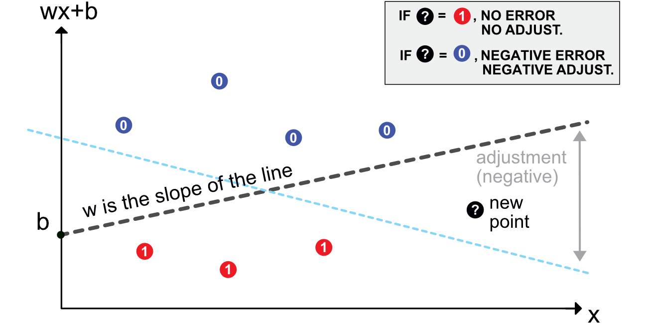
FIGURE 7.1: Scheme of a perceptron.

• if the point is red, there is no need for adjustment: it is labelled correctly as it lies on the right side of the border.
  
• if the point is blue, then the model needs to be updated appropriately. Given the rule mentioned above, this means adjusting the slope of the line downwards. Depending on \(\eta\), the shift will be sufficient to change the classification of the new point - or not.

At the time of its inception, the perceptron was an immense breakthrough which received an intense media coverage (see Olazaran (1996) and Anderson and Rosenfeld (2000)). Its rather simple structure was progressively generalized to networks (combinations) of perceptrons. Each one of them is a simple unit, and units are gathered into layers. The next section describes the organization of simple multilayer perceptrons (MLPs).

7.2 Multilayer perceptron

7.2.1 Introduction and notations

A perceptron can be viewed as a linear model to which is applied a particular function: the Heaviside (step) function. Other choices of functions are naturally possible. In the NN jargon, they are called activation functions. Their purpose is to introduce nonlinearity in otherwise very linear models.

Just like for random forests with trees, the idea behind neural networks is to combine perceptron-like building blocks. A popular representation of neural networks is shown in Figure 7.2. This scheme is overly simplistic. It hides what is really going on: there is a perceptron in each green circle and each output is activated by some function before it is sent to the final output aggregation. This is why such a model is called a Multilayer Perceptron (MLP).

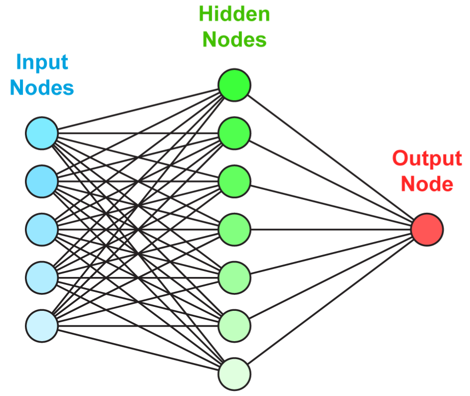
FIGURE 7.2: Simplified scheme of a multi-layer perceptron.

A more faithful account of what is going on is laid out in Figure 7.3.

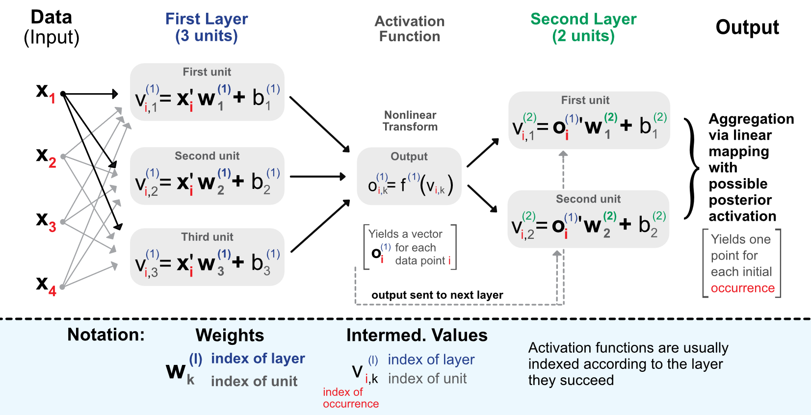
FIGURE 7.3: Detailed scheme of a perceptron with 2 intermediate layers.

Before we proceed with comments, we introduce some notation that will be used thoughout the chapter.

• The data is separated into a matrix \(\textbf{X}=x_{i,j}\) of features and a vector of output values \(\textbf{y}=y_i\). \(\textbf{x}\) or \(\textbf{x}_i\) denotes one line of \(\textbf{X}\).
• A neural network will have \(L\ge1\) layers and for each layer \(l\), the number of units is \(U_l\ge1\).
• The weights for unit \(k\) located in layer \(l\) are denoted with \(\textbf{w}_{k}^{(l)}=w_{k,j}^{(l)}\) and the corresponding biases \(b_{k}^{(l)}\). The length of \(\textbf{w}_{k}^{(l)}\) is equal to \(U_{l-1}\). \(k\) refers to the location of the unit in layer \(l\) while \(j\) to the unit in layer \(l-1\).
• Outputs (post-activation) are denoted \(o_{i,k}^{(l)}\) for instance \(i\), layer \(l\) and unit \(k\).

The process is the following. When entering the network, the data goes though the initial linear mapping:
\[v_{i,k}^{(1)}=\textbf{x}_i'\textbf{w}^{(1)}_k+b_k^{(1)}, \text{for } l=1, \quad k \in [1,U_1], \]
which is then transformed by a non-linear function \(f^{1}\). The result of this alteration is then given as input of the next layer and so on. The linear forms will be repeated (with different weights) for each layer of the network: \[v_{i,k}^{(l)}=(\textbf{o}^{(l-1)}_i)'\textbf{w}^{(l)}_k+b_k^{(l)}, \text{for } l \ge 2, \quad k \in [1,U_l]. \]
The connections between the layers are the so-called outputs, which are basically the linear mappings to which the activation functions \(f^{(l)}\) have been applied. The output of layer \(l\) is the input of layer \(l+1\). \[o_{i,k}^{(l)}=f^{(l)}\left(v_{i,k}^{(l)}\right).\]
Finally, the terminal stage aggregates the outputs from the last layer:
\[\tilde{y}_i =f^{(L+1)} \left((\textbf{o}^{(L)}_i)'\textbf{w}^{(L+1)}+b^{(L+1)}\right).\]

In the forward-propagation of the input, the activation function naturally plays an important role. In Figure 7.4, we plot the most usual activation functions used by neural network libraries. For an exhaustive list of activation functions, we refer to Dubey, Singh, and Chaudhuri (2022).

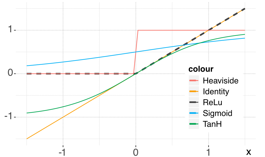
FIGURE 7.4: Plot of the most common activation functions.

Let us rephrase the process through the lens of factor investing. The input \(\textbf{x}\) are the characteristics of the firms. The first step is to multiply their value by weights and add a bias. This is performed for all the units of the first layer. The output, which is a linear combination of the input is then transformed by the activation function. Each unit provides one value and all of these values are fed to the second layer following the same process. This is iterated until the end of the network. The purpose of the last layer is to yield an output shape that corresponds to the label: if the label is numerical, the output is a single number, if it is categorical, then usually it is a vector with length equal to the number of categories. This vector indicates the probability that the value belongs to one particular category.

It is possible to use a final activation function after the output. This can have a huge importance on the result. Indeed, if the labels are returns, applying a sigmoid function at the very end will be disastrous because the sigmoid is always positive.

7.2.2 Universal approximation

One reason neural networks work well is that they are universal approximators. Given any bounded continuous function, there exists a one-layer network that can approximate this function up to arbitrary precision (see Cybenko (1989) for early references, section 4.2 in K.-L. Du and Swamy (2013) and section 6.4.1 in Goodfellow et al. (2016) for more exhaustive lists of papers, and Guliyev and Ismailov (2018) for recent results).

Formally, a one-layer perceptron is defined by \[f_n(\textbf{x})=\sum_{l=1}^nc_l\phi(\textbf{x}\textbf{w}_l+\textbf{b}_l)+c_0,\] where \(\phi\) is a (non-constant) bounded continuous function. Then, for any \(\epsilon>0\), it is possible to find one \(n\) such that for any continuous function \(f\) on the unit hypercube \([0,1]^d\), \[|f(\textbf{x})-f_n(\textbf{x})|< \epsilon, \quad \forall \textbf{x} \in [0,1]^d.\]

This result is rather intuitive: it suffices to add units to the layer to improve the fit. The process is more or less analogous to polynomial approximation, though some subtleties arise depending on the properties of the activation functions (boundedness, smoothness, convexity, etc.). We refer to Costarelli, Spigler, and Vinti (2016) for a survey on this topic.

The raw results on universal approximation imply that any well-behaved function \(f\) can be approached sufficiently closely by a simple neural network, as long as the number of units can be arbitrarily large. Now, they do not directly relate to the learning phase, i.e., when the model is optimized with respect to a particular dataset. In a series of papers (Barron (1993) and Barron (1994), notably), Barron gives a much more precise characterization of what neural networks can achieve. In Barron (1993) it is for instance proved a more precise version of universal approximation: for particular neural networks (with sigmoid activation), \(\mathbb{E}[(f(\textbf{x})-f_n(\textbf{x}))^2]\le c_f/n\), which gives a speed of convergence related to the size of the network. In the expectation, the random term is \(\textbf{x}\): this corresponds to the case where the data is considered to be a sample of i.i.d. observations of a fixed distribution (this is the most common assumption in machine learning).

Below, we state one important result that is easy to interpret; it is taken from Barron (1994).

In the sequel, \(f_n\) corresponds to a possibly penalized neural network with only one intermediate layer with \(n\) units and sigmoid activation function. Moreover, both the supports of the predictors and the label are assumed to be bounded (which is not a major constraint). The most important metric in a regression exercise is the mean squared error (MSE) and the main result is a bound (in order of magnitude) on this quantity. For \(N\) randomly sampled i.i.d. points \(y_i=f(x_i)+\epsilon_i\) on which \(f_n\) is trained, the best possible empirical MSE behaves like

\[\begin{equation} \tag{7.1} \mathbb{E}\left[(f(x)-f_n(x))^2 \right]=\underbrace{O\left(\frac{c_f}{n} \right)}_{\text{size of network}}+\ \underbrace{O\left(\frac{nK \log(N)}{N} \right)}_{\text{size of sample}}, \end{equation}\] where \(K\) is the dimension of the input (number of columns) and \(c_f\) is a constant that depends on the generator function \(f\). The above quantity provides a bound on the error that can be achieved by the best possible neural network given a dataset of size \(N\).

There are clearly two components in the decomposition of this bound. The first one pertains to the complexity of the network. Just as in the original universal approximation theorem, the error decreases with the number of units in the network. But this is not enough! Indeed, the sample size is of course a key driver in the quality of learning (of i.i.d. observations). The second component of the bound indicates that the error decreases at a slightly slower pace with respect to the number of observations (\(\log(N)/N\)) and is linear in the number of units and the size of the input. This clearly underlines the link (trade-off?) between sample size and model complexity: having a very complex model is useless if the sample is small just like a simple model will not catch the fine relationships in a large dataset.

Overall, a neural network is a possibly very complicated function with a lot of parameters. In linear regressions, it is possible to increase the fit by spuriously adding exogenous variables. In neural networks, it suffices to increase the number of parameters by arbitrarily adding units to the layer(s). This is of course a very bad idea because high-dimensional networks will mostly capture the particularities of the sample they are trained on.

7.2.3 Learning via back-propagation

Just like for tree methods, neural networks are trained by minimizing some loss function subject to some penalization: \[O=\sum_{i=1}^I \text{loss}(y_i,\tilde{y}_i)+ \text{penalization},\] where \(\tilde{y}_i\) are the values obtained by the model and \(y_i\) are the true values of the instances. A simple requirement that eases computation is that the loss function be differentiable. The most common choices are the squared error for regression tasks and cross-entropy for classification tasks. We discuss the technicalities of classification in the next subsection.

The training of a neural network amounts to alter the weights (and biases) of all units in all layers so that \(O\) defined above is the smallest possible. To ease the notation and given that the \(y_i\) are fixed, let us write \(D(\tilde{y}_i(\textbf{W}))=\text{loss}(y_i,\tilde{y}_i)\), where \(\textbf{W}\) denotes the entirety of weights and biases in the network. The updating of the weights will be performed via gradient descent, i.e., via

\[\begin{equation} \tag{7.2} \textbf{W} \leftarrow \textbf{W}-\eta \frac{\partial D(\tilde{y}_i) }{\partial \textbf{W}}. \end{equation}\]

This mechanism is the most classical in the optimization literature and we illustrate it in Figure 7.5. We highlight the possible suboptimality of large learning rates. In the diagram, the descent associated with the high \(\eta\) will oscillate around the optimal point, whereas the one related to the small eta will converge more directly.

The complicated task in the above equation is to compute the gradient (derivative) which tells in which direction the adjustment should be done. The problem is that the successive nested layers and associated activations require many iterations of the chain rule for differentiation.

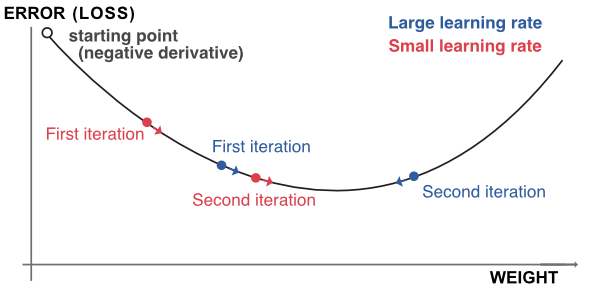
FIGURE 7.5: Outline of gradient descent.

The most common way to approximate a derivative is probably the finite difference method. Under the usual assumptions (the loss is twice differentiable), the centered difference satisfies:

\[\frac{\partial D(\tilde{y}_i(w_k))}{\partial w_k} = \frac{D(\tilde{y}_i(w_k+h))-D(\tilde{y}_i(w_k-h))}{2h}+O(h^2),\] where \(h>0\) is some arbitrarily small number. In spite of its apparent simplicity, this method is costly computationally because it requires a number of operations of the magnitude of the number of weights.

Luckily, there is a small trick that can considerably ease and speed up the computation. The idea is to simply follow the chain rule and recycle terms along the way. Let us start by recalling \[\tilde{y}_i =f^{(L+1)} \left((\textbf{o}^{(L)}_i)'\textbf{w}^{(L+1)}+b^{(L+1)}\right)=f^{(L+1)}\left(b^{(L+1)}+\sum_{k=1}^{U_L} w^{(L+1)}_ko^{(L)}_{i,k} \right),\] so that if we differentiate with the most immediate weights and biases, we get: \[\begin{align} \frac{\partial D(\tilde{y}_i)}{\partial w_k^{(L+1)}}&=D'(\tilde{y}_i) \left(f^{(L+1)} \right)'\left( b^{(L+1)}+\sum_{k=1}^{U_L} w^{(L+1)}_ko^{(L)}_{i,k} \right)o^{(L)}_{i,k} \\ \tag{7.3} &= D'(\tilde{y}_i) \left(f^{(L+1)} \right)'\left( v^{(L+1)}_{i,k} \right)o^{(L)}_{i,k} \\ \frac{\partial D(\tilde{y}_i)}{\partial b^{(L+1)}}&=D'(\tilde{y}_i) \left(f^{(L+1)} \right)'\left( b^{(L+1)}+\sum_{k=1}^{U_L} w^{(L+1)}_ko^{(L)}_{i,k} \right). \end{align}\]

This is the easiest part. We must now go back one layer and this can only be done via the chain rule. To access layer \(L\), we recall identity \(v_{i,k}^{(L)}=(\textbf{o}^{(L-1)}_i)'\textbf{w}^{(L)}_k+b_k^{(L)}=b_k^{(L)}+\sum_{j=1}^{U_L}o^{(L-1)}_{i,j}w^{(L)}_{k,j}\). We can then proceed:

\[\begin{align} \frac{\partial D(\tilde{y}_i)}{\partial w_{k,j}^{(L)}}&=\frac{\partial D(\tilde{y}_i)}{\partial v^{(L)}_{i,k}}\frac{\partial v^{(L)}_{i,k}}{\partial w_{k,j}^{(L)}} = \frac{\partial D(\tilde{y}_i)}{\partial v^{(L)}_{i,k}}o^{(L-1)}_{i,j}\\ &=\frac{\partial D(\tilde{y}_i)}{\partial o^{(L)}_{i,k}} \frac{\partial o^{(L)}_{i,k} }{\partial v^{(L)}_{i,k}} o^{(L-1)}_{i,j} = \frac{\partial D(\tilde{y}_i)}{\partial o^{(L)}_{i,k}} (f^{(L)})'(v_{i,k}^{(L)}) o^{(L-1)}_{i,j} \\ &=\underbrace{D'(\tilde{y}_i) \left(f^{(L+1)} \right)'\left(v^{(L+1)}_{i,k} \right)}_{\text{computed above!}} w^{(L+1)}_k (f^{(L)})'(v_{i,k}^{(L)}) o^{(L-1)}_{i,j}, \end{align}\]

where, as we show in the last line, one part of the derivative was already computed in the previous step (Equation (7.3)). Hence, we can recycle this number and only focus on the right part of the expression.

The magic of the so-called back-propagation is that this will hold true for each step of the differentiation. When computing the gradient for weights and biases in layer \(l\), there will be two parts: one that can be recycled from previous layers and another, local part, that depends only on the values and activation function of the current layer. A nice illustration of this process is given by the Google developer team: playground.tensorflow.org.

When the data is formatted using tensors, it is possible to resort to vectorization so that the number of calls is limited to an order of the magnitude of the number of nodes (units) in the network.

The back-propagation algorithm can be summarized as follows. Given a sample of points (possibly just one):

1. the data flows from left as is described in Figure 7.6. The blue arrows show the forward pass;
   
2. this allows the computation of the error or loss function;
   
3. all derivatives of this function (w.r.t. weights and biases) are computed, starting from the last layer and diffusing to the left (hence the term back-propagation) - the green arrows show the backward pass;
   
4. all weights and biases can be updated to take the sample points into account (the model is adjusted to reduce the loss/error stemming from these points).

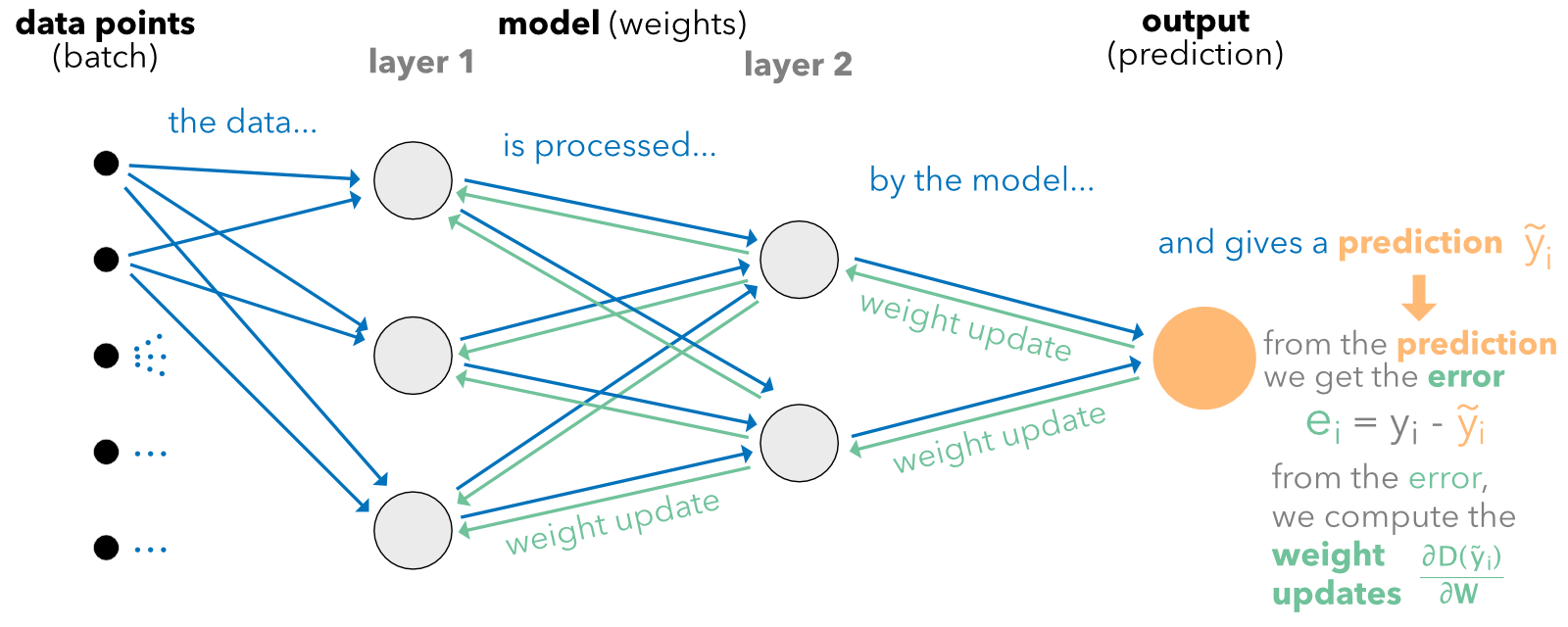
FIGURE 7.6: Diagram of back-propagation.

This operation can be performed any number of times with different sample sizes. We discuss this issue in Section 7.3.

The learning rate \(\eta\) can be refined. One option to reduce overfitting is to impose that after each epoch, the intensity of the update decreases. One possible parametric form is \(\eta=\alpha e^{- \beta t}\), where \(t\) is the epoch and \(\alpha,\beta>0\). One further sophistication is to resort to so-called momentum (which originates from Polyak (1964)): \[\begin{align} \tag{7.4} \textbf{W}_{t+1} & \leftarrow \textbf{W}_{t} - \textbf{m}_t \quad \text{with} \nonumber \\ \textbf{m}_t & \leftarrow \eta \frac{\partial D(\tilde{y}_i)}{\partial \textbf{W}_{t}}+\gamma \textbf{m}_{t-1}, \end{align}\] where \(t\) is the index of the weight update. The idea of momentum is to speed up the convergence by including a memory term of the last adjustment (\(\textbf{m}_{t-1}\)) and going in the same direction in the current update. The parameter \(\gamma\) is often taken to be 0.9.

More complex and enhanced methods have progressively been developed:
- Nesterov (1983) improves the momentum term by forecasting the future shift in parameters;
- Adagrad (Duchi, Hazan, and Singer (2011)) uses a different learning rate for each parameter;
- Adadelta (Zeiler (2012)) and Adam (Kingma and Ba (2014)) combine the ideas of Adagrad and momentum.

Lastly, in some degenerate case, some gradients may explode and push weights far from their optimal values. In order to avoid this phenomenon, learning libraries implement gradient clipping. The user specifies a maximum magnitude for gradients, usually expressed as a norm. Whenever the gradient surpasses this magnitude, it is rescaled to reach the authorized threshold. Thus, the direction remains the same, but the adjustment is smaller.

7.2.4 Further details on classification

In decision trees, the ultimate goal is to create homogeneous clusters, and the process to reach this goal was outlined in the previous chapter. For neural networks, things work differently because the objective is explicitly to minimize the error between the prediction \(\tilde{\textbf{y}}_i\) and a target label \(\textbf{y}_i\). Again, here \(\textbf{y}_i\) is a vector full of zeros with only one one denoting the class of the instance.

Facing a classification problem, the trick is to use an appropriate activation function at the very end of the network. The dimension of the terminal output of the network should be equal to \(J\) (number of classes to predict), and if, for simplicity, we write \(\textbf{x}_i\) for the values of this output, the most commonly used activation is the so-called softmax function:

\[\tilde{\textbf{y}}_i=s(\textbf{x})_i=\frac{e^{x_i}}{\sum_{j=1}^Je^{x_j}}.\]

The justification of this choice is straightforward: it can take any value as input (over the real line) and it sums to one over any (finite-valued) output. Similarly as for trees, this yields a ‘probability’ vector over the classes. Often, the chosen loss is a generalization of the entropy used for trees. Given the target label \(\textbf{y}_i=(y_{i,1},\dots,y_{i,L})=(0,0,\dots,0,1,0,\dots,0)\) and the predicted output \(\tilde{\textbf{y}}_i=(\tilde{y}_{i,1},\dots,\tilde{y}_{i,L})\), the cross-entropy is defined as

\[\begin{equation} \tag{7.5} \text{CE}(\textbf{y}_i,\tilde{\textbf{y}}_i)=-\sum_{j=1}^J\log(\tilde{y}_{i,j})y_{i,j}. \end{equation}\]

Basically, it is a proxy of the dissimilarity between its two arguments. One simple interpretation is the following. For the nonzero label value, the loss is \(-\log(\tilde{y}_{i,l})\), while for all others, it is zero. In the log, the loss will be minimal if \(\tilde{y}_{i,l}=1\), which is exactly what we seek (i.e., \(y_{i,l}=\tilde{y}_{i,l}\)). In applications, this best case scenario will not happen, and the loss will simply increase when \(\tilde{y}_{i,l}\) drifts away downwards from one.

7.3 How deep we should go and other practical issues

Beyond the ones presented in the previous sections, the user faces many degrees of freedom when building a neural network. We present a few classical choices that are available when constructing and training neural networks.

7.3.1 Architectural choices

Arguably, the first choice pertains to the structure of the network. Beyond the dichotomy feed-forward versus recurrent (see Section ??), the immediate question is: how big (or how deep) the networks should be. First of all, let us calculate the number of parameters (i.e., weights plus biases) that are estimated (optimized) in a network.

• For the first layer, this gives \((U_0+1)U_1\) parameters, where \(U_0\) is the number of columns in \(\mathbb{X}\) (i.e., number of explanatory variables) and \(U_1\) is the number of units in the layer.
  
• For layer \(l\in[2,L]\), the number of parameters is \((U_{l-1}+1)U_l\).
  
• For the final output, there are simply \(U_L+1\) parameters.
  
• In total, this means the total number of values to optimize is \[\mathcal{N}=\left(\sum_{l=1}^L(U_{l-1}+1)U_l\right)+U_L+1\]

As in any model, the number of parameters should be much smaller than the number of instances. There is no fixed ratio, but it is preferable if the sample size is at least ten times larger than the number of parameters. Below a ratio of 5, the risk of overfitting is high. Given the amount of data readily available, this constraint is seldom an issue, unless one wishes to work with a very large network.

The number of hidden layers in current financial applications rarely exceeds three or four. The number of units per layer \((U_k)\) is often chosen to follow the geometric pyramid rule (see, e.g., Masters (1993)). If there are \(L\) hidden layers, with \(I\) features in the input and \(O\) dimensions in the output (for regression tasks, \(O=1\)), then, for the \(k^{th}\) layer, a rule of thumb for the number of units is \[U_k\approx \left\lfloor O\left( \frac{I}{O}\right)^{\frac{L+1-k}{L+1}}\right\rfloor.\] If there is only one intermediate layer, the recommended proxy is the integer part of \(\sqrt{IO}\). If not, the network starts with many units and the number of unit decreases exponentially towards the output size. Often, the number of layers is a power of two because, in high dimensions, networks are trained on Graphics Processing Units (GPUs) or Tensor Processing Units (TPUs). Both pieces of hardware can be used optimally when the inputs have sizes equals to powers of two.

Several studies have shown that very large architectures do not always perform better than more shallow ones (e.g., Gu, Kelly, and Xiu (2020b) and Orimoloye et al. (2019) for high frequency data, i.e., not factor-based). As a rule of thumb, a maximum of three hidden layers seem to be sufficient for prediction purposes.

7.3.2 Frequency of weight updates and learning duration

In the expression (7.2), it is implicit that the computation is performed for one given instance. If the sample size is very large (hundreds of thousands or millions of instances), updating the weights according to each point is computationally too costly. The updating is then performed on groups of instances which are called batches. The sample is (randomly) split into batches of fixed sizes and each update is performed following the rule:

\[\begin{equation} \tag{7.6} \textbf{W} \leftarrow \textbf{W}-\eta \frac{\partial \sum_{i \in \text{batch}} D(\tilde{y}_i)/\text{card}(\text{batch}) }{\partial \textbf{W}}. \end{equation}\]

The change in weights is computed over the average loss computed over all instances in the batch. The terminology for training includes:

• epoch: one epoch is reached when each instance of the sample has contributed to the update of the weights (i.e., the training). Often, training a NN requires several epochs and up to a few dozen.
  
• batch size: the batch size is the number of samples used for one single update of weights.
  
• iterations: the number of iterations can mean alternatively the ratio of sample size divided by batch size or this ratio multiplied by the number of epochs. It’s either the number of weight updates required to reach one epoch or the total number of updates during the whole training.

When the batch is equal to only one instance, the method is referred to as ‘stochastic gradient descent’ (SGD): the instance is chosen randomly. When the batch size is strictly above one and below the total number of instances, the learning is performed via ‘mini’ batches, that is, small groups of instances. The batches are also chosen randomly, but without replacement in the sample because for one epoch, the union of batches must be equal to the full training sample.

It is impossible to know in advance what a good number of epochs is. Sometimes, the network stops learning after just 5 epochs (the validation loss does not decrease anymore). In some cases when the validation sample is drawn from a distribution close to that of the training sample, the network continues to learn even after 200 epochs. It is up to the user to test different values to evaluate the learning speed. In the examples below, we keep the number of epochs low for computational purposes.

7.3.3 Penalizations and dropout

At each level (layer), it is possible to enforce constraints or penalizations on the weights (and biases). Just as for tree methods, this helps slow down the learning to prevent overfitting on the training sample. Penalizations are enforced directly on the loss function and the objective function takes the form

\[O=\sum_{i=1}^I \text{loss}(y_i,\tilde{y}_i)+ \sum_{k} \lambda_k||\textbf{W}_k||_1+ \sum_j\delta_j||\textbf{W}_j||_2^2,\] where the subscripts \(k\) and \(j\) pertain to the weights to which the \(L^1\) and (or) \(L^2\) penalization is applied.

In addition, specific constraints can be enforced on the weights directly during the training. Typically, two types of constraints are used:

• norm constraints: a maximum norm is fixed for the weight vectors or matrices;
  
• non-negativity constraint: all weights must be positive or zero.

Lastly, another (somewhat exotic) way to reduce the risk of overfitting is simply to reduce the size (number of parameters) of the model. Srivastava et al. (2014) propose to omit units during training (hence the term ‘dropout’). The weights of randomly chosen units are set to zero during training. All links from and to the unit are ignored, which mechanically shrinks the network. In the testing phase, all units are back, but the values (weights) must be scaled to account for the missing activations during the training phase.

The interested reader can check the advice compiled in Bengio (2012), Hanin and Rolnick (2018), and L. N. Smith (2018) for further tips on how to configure neural networks. A paper dedicated to hyperparameter tuning for stock return prediction is S. I. Lee (2020).

7.4 Code samples and comments for vanilla MLP

There are several frameworks and libraries that allow robust and flexible constructions of neural networks. Among them, Keras and Tensorflow (developed by Google) are probably the most used at the time we write this book (PyTorch, from Facebook, is one alternative). For simplicity and because we believe it is the best choice, we implement the NN with Keras (which is the high level API of Tensorflow, see https://www.tensorflow.org). The original Python implementation is referenced on https://keras.io, and the details for the R version can be found here: https://keras.rstudio.com. We recommend a thorough installation before proceeding. Because the native versions of Tensorflow and Keras are written in Python (and accessed by R via the reticulate package), a running version of Python is required below. To install Keras, please follow the instructions provided at https://keras.rstudio.com.

In this section, we provide a detailed (though far from exhaustive) account of how to train neural networks with Keras. For the sake of completeness, we proceed in two steps. The first one relates to a very simple regression exercise. Its purpose is to get the reader familiar with the syntax of Keras. In the second step, we lay out many of the options proposed by Keras to perform a classification exercise. With these two examples, we thus cover most of the mainstream topics falling under the umbrella of feed-forward multilayered perceptrons.

7.4.1 Regression example

Before we head to the core of the NN, a short stage of data preparation is required. Just as for penalized regressions (glmnet package) and boosted trees (xgboost package), the data must be sorted into four parts which are the combination of two dichotomies: training versus testing and labels versus features. We define the corresponding variables below. For simplicity, the first example is a regression exercise. A classification task will be detailed below.

NN_train_features <- dplyr::select(training_sample, features) %>%    # Training features
  as.matrix()                                                      # Matrix = important
NN_train_labels <- training_sample$R1M_Usd                           # Training labels
NN_test_features <- dplyr::select(testing_sample, features) %>%      # Testing features
  as.matrix()                                                      # Matrix = important
NN_test_labels <- testing_sample$R1M_Usd                             # Testing labels

In Keras, the training of neural networks is performed through three steps:

1. Defining the structure/architecture of the network;
   
2. Setting the loss function and learning process (options on the updating of weights);
   
3. Train by specifying the batch sizes and number of rounds (epochs).

We start with a very simple architecture with two hidden layers.

library(keras)
# install_keras() # To complete installation
model <- keras_model_sequential()
model %>%   # This defines the structure of the network, i.e. how layers are organized
  layer_dense(units = 16, activation = 'relu', input_shape = ncol(NN_train_features)) %>%
  layer_dense(units = 8, activation = 'tanh') %>%
  layer_dense(units = 1) # No activation means linear activation: f(x) = x.

The definition of the structure is very intuitive and uses the sequential syntax in which one input is iteratively transformed by a layer until the last iteration which gives the output. Each layer depends on two parameters: the number of units and the activation function that is applied to the output of the layer. One important point is the input_shape parameter for the first layer. It is required for the first layer and is equal to the number of features. For the subsequent layers, the input_shape is dictated by the number of units of the previous layer; hence it is not required. The activations that are currently available are listed on https://keras.io/activations/. We use the hyperbolic tangent in the second-to-last layer because it yields both positive and negative outputs. Of course, the last layer can generate negative values as well, but it’s preferable to satisfy this property one step ahead of the final output.

model %>% compile(                             # Model specification
  loss = 'mean_squared_error',               # Loss function
  optimizer = optimizer_rmsprop(),           # Optimisation method (weight updating)
  metrics = c('mean_absolute_error')         # Output metric
)
summary(model)                                 # Model architecture

## Model: "sequential"
## __________________________________________________________________________________________
## Layer (type)                            Output Shape                        Param #       
## ==========================================================================================
## dense_2 (Dense)                         (None, 16)                          1504          
## __________________________________________________________________________________________
## dense_1 (Dense)                         (None, 8)                           136           
## __________________________________________________________________________________________
## dense (Dense)                           (None, 1)                           9             
## ==========================================================================================
## Total params: 1,649
## Trainable params: 1,649
## Non-trainable params: 0
## __________________________________________________________________________________________

The summary of the model lists the layers in their order from input to output (forward pass). Because we are working with 93 features, the number of parameters for the first layer (16 units) is 93 plus one (for the bias) multiplied by 16, which makes 1504. For the second layer, the number of inputs is equal to the size of the output from the previous layer (16). Hence given the fact that the second layer has 8 units, the total number of parameters is (16+1)*8 = 136.

We set the loss function to the standard mean squared error. Other losses are listed on https://keras.io/losses/, some of them work only for regressions (MSE, MAE) and others only for classification (categorical cross-entropy, see Equation (7.5)). The RMS propragation optimizer is the classical mini-batch back-propagation implementation. For other weight updating algorithms, we refer to https://keras.io/optimizers/. The metric is the function used to assess the quality of the model. It can be different from the loss: for instance, using entropy for training and accuracy as the performance metric.

The final stage fits the model to the data and requires some additional training parameters:

fit_NN <- model %>% 
  fit(NN_train_features,                                       # Training features
      NN_train_labels,                                         # Training labels
      epochs = 10, batch_size = 512,                           # Training parameters
      validation_data = list(NN_test_features, NN_test_labels) # Test data
  ) 
plot(fit_NN) + theme_light()                                   # Plot, evidently!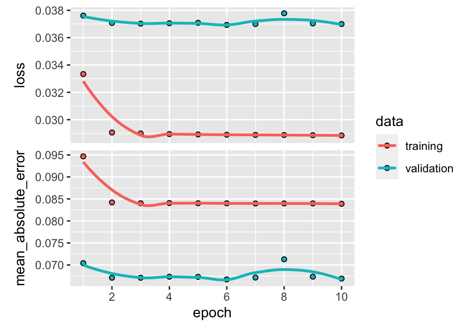

FIGURE 7.7: Output from a trained neural network (regression task).

The batch size is quite arbitrary. For technical reasons pertaining to training on GPUs, these sizes are often powers of 2.

In Keras, the plot of the trained model shows four different curves (shown here in Figure 7.7). The top graph displays the improvement (or lack thereof) in loss as the number of epochs increases. Usually, the algorithm starts by learning rapidly and then converges to a point where any additional epoch does not improve the fit. In the example above, this point arrives rather quickly because it is hard to notice any gain beyond the fourth epoch. The two colors show the performance on the two samples: the training sample and the testing sample. By construction, the loss will always improve (even marginally) on the training sample. When the impact is negligible on the testing sample (the curve is flat, as is the case here), the model fails to generalize out-of-sample: the gains obtained by training on the original sample do not translate to gains on previously unseen data; thus, the model seems to be learning noise.

The second graph shows the same behavior but is computed using the metric function. The correlation (in absolute terms) between the two curves (loss and metric) is usually high. If one of them is flat, the other should be as well.

In order to obtain the parameters of the model, the user can call get_weights(model).¹⁸ We do not execute the code here because the size of the output is much too large, as there are thousands of weights.

Finally, from a practical point of view, the prediction is obtained via the usual predict() function. We use this function below on the testing sample to calculate the hit ratio.

mean(predict(model, NN_test_features) * NN_test_labels > 0) # Hit ratio

## [1] 0.5456358

Again, the hit ratio lies between 50% and 55%, which seems reasonably good. Most of the time, neural networks have their weights initialized randomly. Hence, two independently trained networks with the same architecture and same training data may well lead to very different predictions and performance! One way to bypass this issue is to freeze the random number generator. Models can also be easily exchanged by loading weights via the set_weights() function.

7.4.2 Classification example

We pursue our exploration of neural networks with a much more detailed example. The aim is to carry out a classification task on the binary label R1M_Usd_C. Before we proceed, we need to format the label properly. To this purpose, we resort to one-hot encoding (see Section 4.5.2).

library(dummies)                                            # Package for one-hot encoding
NN_train_labels_C <- training_sample$R1M_Usd_C %>% dummy()  # One-hot encoding of the label
NN_test_labels_C <- testing_sample$R1M_Usd_C %>% dummy()    # One-hot encoding of the label

The labels NN_train_labels_C and NN_test_labels_C have two columns: the first flags the instances with above median returns and the second flags those with below median returns. Note that we do not alter the feature variables: they remain unchanged. Below, we set the structure of the networks with many additional features compared to the first one.

model_C <- keras_model_sequential()
model_C %>%   # This defines the structure of the network, i.e. how layers are organized
  layer_dense(units = 16, activation = 'tanh',               # Nb units & activation
              input_shape = ncol(NN_train_features),         # Size of input
              kernel_initializer = "random_normal",          # Initialization of weights
              kernel_constraint = constraint_nonneg()) %>%   # Weights should be nonneg
  layer_dropout(rate = 0.25) %>%                             # Dropping out 25% units
  layer_dense(units = 8, activation = 'elu',                 # Nb units & activation
              bias_initializer = initializer_constant(0.2),  # Initialization of biases
              kernel_regularizer = regularizer_l2(0.01)) %>% # Penalization of weights 
  layer_dense(units = 2, activation = 'softmax')             # Softmax for categorical output

Before we start commenting on the many options used above, we highlight that Keras models, unlike many R variables, are mutable objects. This means that any piping %>% after calling a model will alter it. Hence, successive trainings do not start from scratch but from the result of the previous training.

First, the options used above and below were chosen as illustrative examples and do not serve to particularly improve the quality of the model. The first change compared to Section 7.4.1 is the activation functions. The first two are simply new cases, while the third one (for the output layer) is imperative. Indeed, since the goal is classification, the dimension of the output must be equal to the number of categories of the labels. The activation that yields a multivariate is the softmax function. Note that we must also specify the number of classes (categories) in the terminal layer.

The second major innovation is options pertaining to parameters. One family of options deals with the initialization of weights and biases. In Keras, weights are referred to as the ‘kernel’. The list of initializers is quite long and we suggest the interested reader has a look at the Keras reference (https://keras.io/initializers/). Most of them are random, but some of them are constant.

Another family of options is the constraints and norm penalization that are applied on the weights and biases during training. In the above example, the weights of the first layer are coerced to be non-negative, while the weights of the second layer see their magnitude penalized by a factor (0.01) times their \(L^2\) norm.

Lastly, the final novelty is the dropout layer (see Section 7.3.3) between the first and second layers. According to this layer, one fourth of the units in the first layer will be (randomly) omitted during training.

The specification of the training is outlined below.

model_C %>% compile(                               # Model specification
  loss = 'binary_crossentropy',                  # Loss function
  optimizer = optimizer_adam(lr = 0.005,         # Optimisation method (weight updating)
                             beta_1 = 0.9, 
                             beta_2 = 0.95),        
  metrics = c('categorical_accuracy')            # Output metric
)
summary(model_C)                                   # Model structure

## Model: "sequential_1"
## __________________________________________________________________________________________
## Layer (type)                            Output Shape                        Param #       
## ==========================================================================================
## dense_5 (Dense)                         (None, 16)                          1504          
## __________________________________________________________________________________________
## dropout (Dropout)                       (None, 16)                          0             
## __________________________________________________________________________________________
## dense_4 (Dense)                         (None, 8)                           136           
## __________________________________________________________________________________________
## dense_3 (Dense)                         (None, 2)                           18            
## ==========================================================================================
## Total params: 1,658
## Trainable params: 1,658
## Non-trainable params: 0
## __________________________________________________________________________________________

Here again, many changes have been made: all levels have been revised. The loss is now the cross-entropy. Because we work with two categories, we resort to a specific choice (binary cross-entropy), but the more general form is the option categorical_crossentropy and works for any number of classes (strictly above 1). The optimizer is also different and allows for several parameters and we refer to Kingma and Ba (2014). Simply put, the two beta parameters control decay rates for exponentially weighted moving averages used in the update of weights. The two averages are estimates for the first and second moment of the gradient and can be exploited to increase the speed of learning. The performance metric in the above chunk is the categorical accuracy. In multiclass classification, the accuracy is defined as the average accuracy over all classes and all predictions. Since a prediction for one instance is a vector of weights, the ‘terminal’ prediction is the class that is associated with the largest weight. The accuracy then measures the proportion of times when the prediction is equal to the realized value (i.e., when the class is correctly guessed by the model).

Finally, we proceed with the training of the model.

fit_NN_C <- model_C %>% 
  fit(NN_train_features,                                   # Training features
      NN_train_labels_C,                                   # Training labels
      epochs = 20, batch_size = 512,                       # Training parameters
      validation_data = list(NN_test_features, 
                             NN_test_labels_C),            # Test data
      verbose = 0,                                         # No comments from algo
      callbacks = list(
        callback_early_stopping(monitor = "val_loss",    # Early stopping:
                                min_delta = 0.001,       # Improvement threshold
                                patience = 3,            # Nb epochs with no improvmt 
                                verbose = 0              # No warnings
        )
      )
  )
plot(fit_NN_C) + theme_light()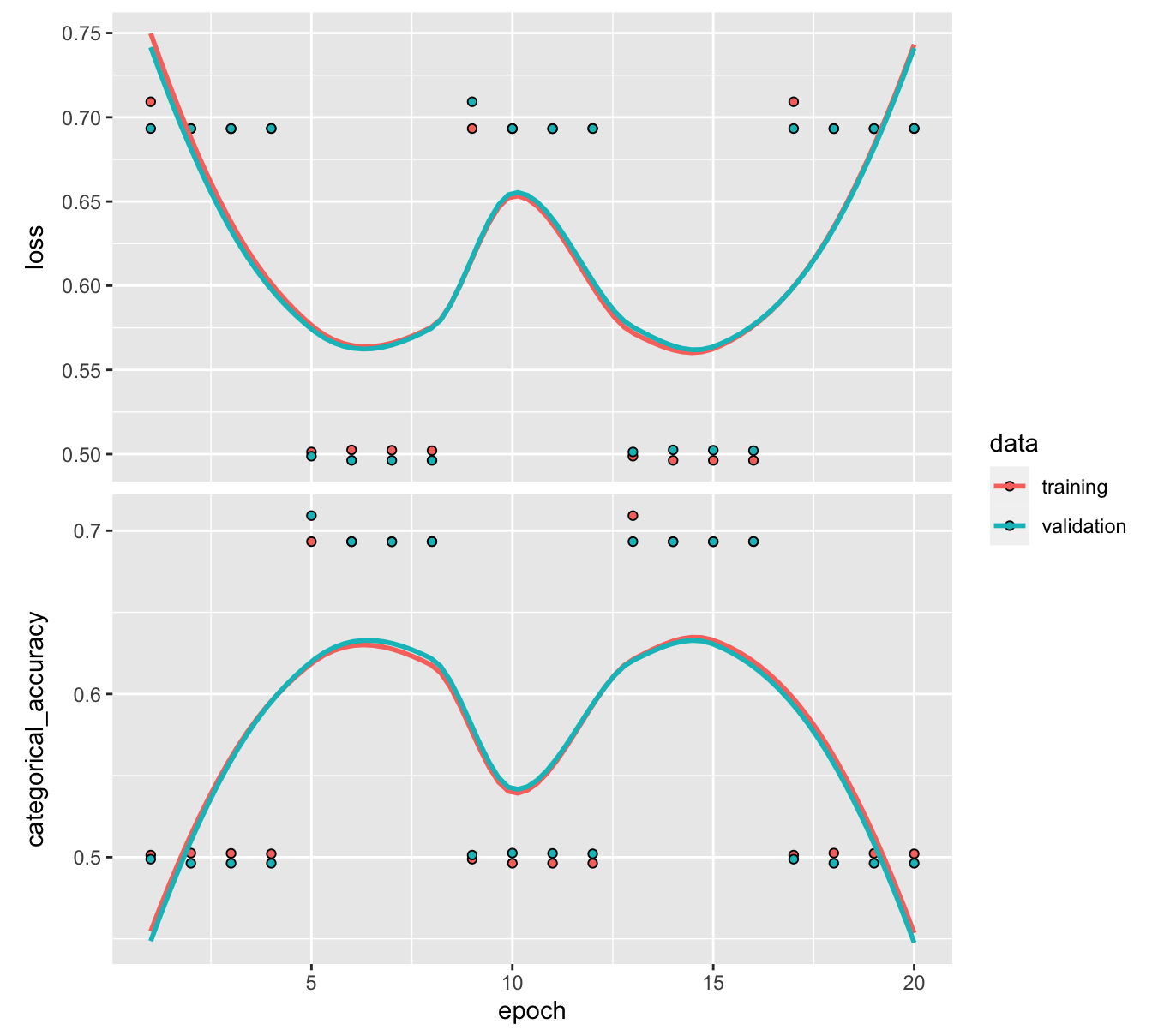

FIGURE 7.8: Output from a trained neural network (classification task) with early stopping.

There is only one major difference here compared to the previous training call. In Keras, callbacks are functions that can be used at given stages of the learning process. In the above example, we use one such function to stop the algorithm when no progress has been made for some time.

When datasets are large, the training can be long, especially when batch sizes are small and/or the number of epochs is high. It is not guaranteed that going to the full number of epochs is useful, as the loss or metric functions may be plateauing much sooner. Hence, it can be very convenient to stop the process if no improvement is achieved during a specified time-frame. We set the number of epochs to 20, but the process will likely stop before that.

In the above code, the improvement is focused on validation accuracy (“val_loss”; one alternative is “val_acc”). The min_delta value sets the minimum improvement that needs to be attained for the algorithm to continue. Therefore, unless the validation accuracy gains 0.001 points at each epoch, the training will stop. Nevertheless, some flexibility is introduced via the patience parameter, which in our case asserts that the halting decision is made only after three consecutive epochs with no improvement. In the option, the verbose parameter dictates the amount of comments that is made by the function. For simplicity, we do not want any comments, hence this value is set to zero.

In Figure 7.8, the two graphs yield very different curves. One reason for that is the scale of the second graph. The range of accuracies is very narrow. Any change in this range does not represent much variation overall. The pattern is relatively clear on the training sample: the loss decreases, while the accuracy improves. Unfortunately, this does not translate to the testing sample which indicates that the model does not generalize well out-of-sample.

7.4.3 Custom losses

In Keras, it is possible to define user-specified loss functions. This may be interesting in some cases. For instance, the quadratic error has three terms \(y_i^2\), \(\tilde{y}_i^2\) and \(-2y_i\tilde{y}_i\). In practice, it can make sense to focus more on the latter term because it is the most essential: we do want predictions and realized values to have the same sign! Below we show how to optimize on a simple (product) function in Keras, \(l(y_i,\tilde{y}_i)=(\tilde{y}_i-\tilde{m})^2-\gamma (y_i-m)(\tilde{y}_i-\tilde{m})\), where \(m\) and \(\tilde{m}\) are the sample averages of \(y_i\) and \(\tilde{y}_i\). With \(\gamma>2\), we give more weight to the cross term. We start with a simple architecture.

model_custom <- keras_model_sequential()
model_custom %>%   # This defines the structure of the network, i.e. how layers are organized
  layer_dense(units = 16, activation = 'relu', input_shape = ncol(NN_train_features)) %>%
  layer_dense(units = 8, activation = 'sigmoid') %>%
  layer_dense(units = 1) # No activation means linear activation: f(x) = x.

Then we code the loss function and integrate it to the model. The important trick is to resort to functions that are specific to the library (the k_functions). We code the variance of predicted values minus the scaled covariance between realized and predicted values. Below we use a scale of five.

# Defines the loss, we use gamma = 5
metric_cust <- custom_metric("custom_loss", 
                             function(y_true, y_pred) {
                               k_mean((y_pred - k_mean(y_pred))*(y_pred - k_mean(y_pred)))-5*k_mean((y_true - k_mean(y_true))*(y_pred - k_mean(y_pred)))
                             })

model_custom %>% compile(                                          # Model specification
  loss =  metric_cust, #function(y_true, y_pred) custom_loss(y_true, y_pred),  # New loss function!
  optimizer = optimizer_rmsprop(),                               # Optim method 
  metrics = c('mean_absolute_error')                             # Output metric
)

Finally, we are ready to train and briefly evaluate the performance of the model.

fit_NN_cust <- model_custom %>% 
  fit(NN_train_features,                                       # Training features
      NN_train_labels,                                         # Training labels
      epochs = 10, batch_size = 512,                           # Training parameters
      validation_data = list(NN_test_features, NN_test_labels) # Test data
  ) 
plot(fit_NN_cust) + theme_light()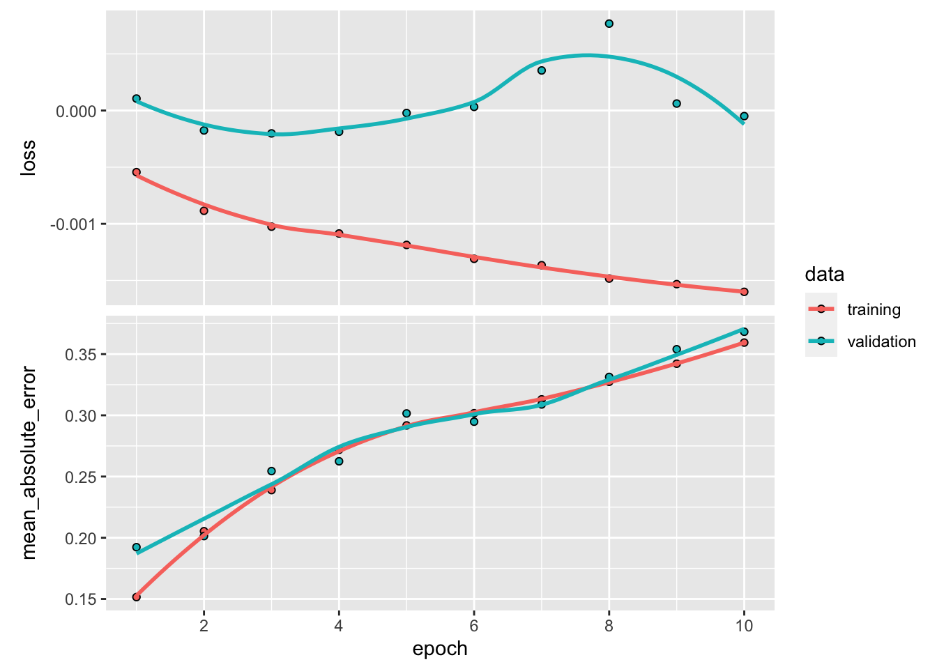  

The curves may go in opposite direction. One reason for that is that while improving correlation between realized and predicted values, we are also increasing the sum of squared predicted returns.

mean(predict(model_custom, NN_test_features) * NN_test_labels > 0) # Hit ratio

## [1] 0.4469434

The outcome could be improved. There are several directions that could help. One of them is arguably that the model should be dynamic and not static (see Chapter 12).

7.5 Recurrent networks

7.5.1 Presentation

Multilayer perceptrons are feed-forward networks because the data flows from left to right with no looping in between. For some particular tasks with sequential linkages (e.g., time-series or speech recognition), it might be useful to keep track of what happened with the previous sample (i.e., there is a natural ordering). One simple way to model ‘memory’ would be to consider the following network with only one intermediate layer: \[\begin{align*} \tilde{y}_i&=f^{(y)}\left(\sum_{j=1}^{U_1}h_{i,j}w^{(y)}_j+b^{(2)}\right) \\ \textbf{h}_{i} &=f^{(h)}\left(\sum_{k=1}^{U_0}x_{i,k}w^{(h,1)}_k+b^{(1)}+ \underbrace{\sum_{k=1}^{U_1} w^{(h,2)}_{k}h_{i-1,k}}_{\text{memory part}} \right), \end{align*}\]

where \(h_0\) is customarily set at zero (vector-wise).

These kinds of models are often referred to as Elman (1990) models or to Jordan (1997) models if in the latter case \(h_{i-1}\) is replaced by \(y_{i-1}\) in the computation of \(h_i\). Both types of models fall under the overarching umbrella of Recurrent Neural Networks (RNNs).

The \(h_i\) is usually called the state or the hidden layer. The training of this model is complicated and must be done by unfolding the network over all instances to obtain a simple feed-forward network and train it regularly. We illustrate the unfolding principle in Figure 7.9. It shows a very deep network. The first input impacts the first layer and then the second one via \(h_1\) and all following layers in the same fashion. Likewise, the second input impacts all layers except the first and each instance \(i-1\) is going to impact the output \(\tilde{y}_i\) and all outputs \(\tilde{y}_j\) for \(j \ge i\). In Figure 7.9, the parameters that are trained are shown in blue. They appear many times, in fact, at each level of the unfolded network.

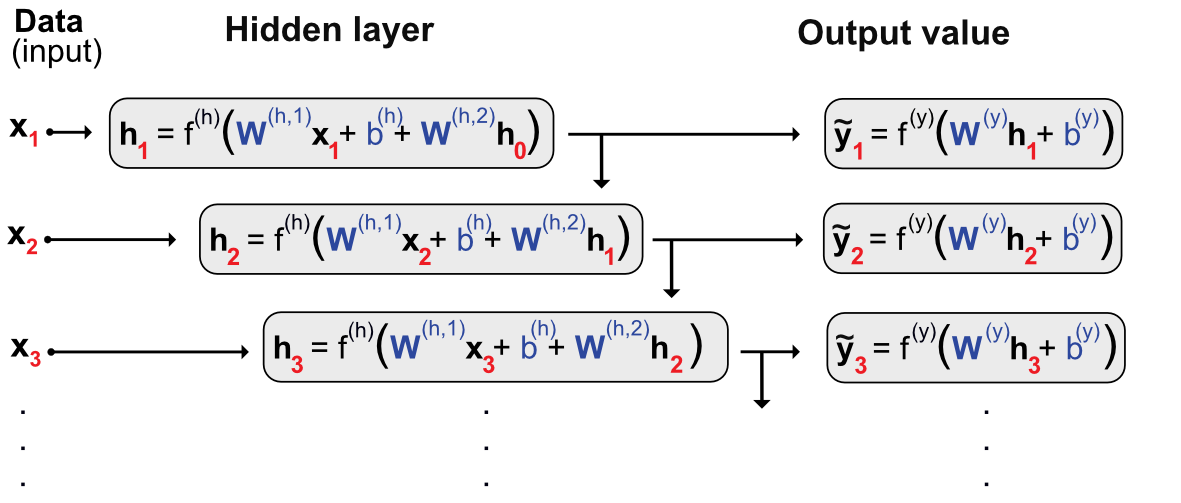
FIGURE 7.9: Unfolding a recurrent network.

The main problem with the above architecture is the loss of memory induced by vanishing gradients. Because of the depth of the model, the chain rule used in the back-propagation will imply a large number of products of derivatives of activation functions. Now, as is shown in Figure 7.4, these functions are very smooth and their derivatives are most of the time smaller than one (in absolute value). Hence, multiplying many numbers smaller than one leads to very small figures: beyond some layers, the learning does not propagate because the adjustments are too small.

One way to prevent this progressive discounting of the memory was introduced in Hochreiter and Schmidhuber (1997) (Long-Short Term Memory - LSTM model). This model was subsequently simplified by the authors Chung et al. (2015) and we present this more parsimonious model below. The Gated Recurrent Unit (GRU) is a slightly more complicated version of the vanilla recurrent network defined above. It has the following representation: \[\begin{align*} \tilde{y}_i&=z_i\tilde{y}_{i-1}+ (1-z_i)\tanh \left(\textbf{w}_y'\textbf{x}_i+ b_y+ u_yr_i\tilde{y}_{i-1}\right) \quad \text{output (prediction)} \\ z_i &= \text{sig}(\textbf{w}_z'\textbf{x}_i+b_z+u_z\tilde{y}_{i-1}) \hspace{9mm} \text{`update gate'} \ \in (0,1)\\ r_i &= \text{sig}(\textbf{w}_r'\textbf{x}_i+b_r+u_r\tilde{y}_{i-1}) \hspace{9mm} \text{`reset gate'} \ \in (0,1). \end{align*}\] In compact form, this gives \[\tilde{y}_i=\underbrace{z_i}_{\text{weight}}\underbrace{\tilde{y}_{i-1}}_{\text{past value}}+ \underbrace{(1-z_i)}_{\text{weight}}\underbrace{\tanh \left(\textbf{w}_y'\textbf{x}_i+ b_y+ u_yr_i\tilde{y}_{i-1}\right)}_{\text{candidate value (classical RNN)}}, \]

where the \(z_i\) decides the optimal mix between the current and past values. For the candidate value, \(r_i\) decides which amount of past/memory to retain. \(r_i\) is commonly referred to as the ‘reset gate’ and \(z_i\) to the ‘update gate’.

There are some subtleties in the training of a recurrent network. Indeed, because of the chaining between the instances, each batch must correspond to a coherent time series. A logical choice is thus one batch per asset with instances (logically) chronologically ordered. Lastly, one option in some frameworks is to keep some memory between the batches by passing the final value of \(\tilde{y}_i\) to the next batch (for which it will be \(\tilde{y}_0\)). This is often referred to as the stateful mode and should be considered meticulously. It does not seem desirable in a portfolio prediction setting if the batch size corresponds to all observations for each asset: there is no particular link between assets. If the dataset is divided into several parts for each given asset, then the training must be handled very cautiously.

Reccurrent networks and LSTM especially have been found to be good forecasting tools in financial contexts (see, e.g., Fischer and Krauss (2018), W. Wang et al. (2020), and Fister, Perc, and Jagrič (2021)).

7.5.2 Code and results

Recurrent networks are theoretically more complicated compared to multilayered perceptrons. In practice, they are also more challenging in their implementation. Indeed, the serial linkages require more attention compared to feed-forward architectures. In an asset pricing framework, we must separate the assets because the stock-specific time series cannot be bundled together. The learning will be sequential, one stock at a time.

The dimensions of variables are crucial. In Keras, they are defined for RNNs as:

1. The size of the batch: in our case, it will be the number of assets. Indeed, the recurrence relationship holds at the asset level, hence each asset will represent a new batch on which the model will learn.
   
2. The time steps: in our case, it will simply be the number of dates.
   
3. The number of features: in our case, there is only one possible figure which is the number of predictors.

For simplicity and in order to reduce computation times, we will use the same subset of stocks as that from Section 5.2.2. This yields a perfectly rectangular dataset in which all dates have the same number of observations.

First, we create some new, intermediate variables.

data_rnn <- data_ml %>%                                  # Dedicated dataset
  filter(stock_id %in% stock_ids_short)
training_sample_rnn <- filter(data_rnn, date < separation_date)
testing_sample_rnn <- filter(data_rnn, date > separation_date)
nb_stocks <- length(stock_ids_short)                     # Nb stocks 
nb_feats <- length(features)                             # Nb features
nb_dates_train <- nrow(training_sample) / nb_stocks      # Nb training dates (size of sample)
nb_dates_test <- nrow(testing_sample) / nb_stocks        # Nb testing dates

Then, we construct the variables we will pass as arguments. We recall that the data file was ordered first by stocks and then by date (see Section 1.2).

train_features_rnn <- array(NN_train_features,           # Formats the training data into array
                            dim = c(nb_dates_train, nb_stocks, nb_feats)) %>% # Tricky order
  aperm(c(2,1,3))                                      # The order is: stock, date, feature 
test_features_rnn <- array(NN_test_features,             # Formats the testing data into array
                           dim = c(nb_dates_test, nb_stocks, nb_feats)) %>%  # Tricky order
  aperm(c(2,1,3))                                      # The order is: stock, date, feature 
train_labels_rnn <- as.matrix(NN_train_labels) %>% 
  array(dim = c(nb_dates_train, nb_stocks, 1)) %>% aperm(c(2,1,3))
test_labels_rnn <- as.matrix(NN_test_labels) %>% 
  array(dim = c(nb_dates_test, nb_stocks, 1)) %>% aperm(c(2,1,3))

Finally, we move towards the training part. For simplicity, we only consider a simple RNN with only one layer. The structure is outlined below. In terms of recurrence structure, we pick a Gated Recurrent Unit (GRU).

model_RNN <- keras_model_sequential() %>% 
  layer_gru(units = 16,                              # Nb units in hidden layer
            batch_input_shape = c(nb_stocks,         # Dimensions = tricky part!
                                  nb_dates_train, 
                                  nb_feats), 
            activation = 'tanh',                     # Activation function
            return_sequences = TRUE) %>%             # Return all the sequence
  layer_dense(units = 1)                             # Final aggregation layer
model_RNN %>% compile(
  loss = 'mean_squared_error',                       # Loss = quadratic
  optimizer = optimizer_rmsprop(),                   # Backprop
  metrics = c('mean_absolute_error')                 # Output metric MAE
)

There are many options available for recurrent layers. For GRUs, we refer to the Keras documentation https://keras.rstudio.com/reference/layer_gru.html. We comment briefly on the option return_sequences which we activate. In many cases, the output is simply the terminal value of the sequence. If we do not require the entirety of the sequence to be returned, we will face a problem in the dimensionality because the label is indeed a full sequence. Once the structure is determined, we can move forward to the training stage.

fit_RNN <- model_RNN %>% fit(train_features_rnn,   # Training features        
                             train_labels_rnn,                # Training labels
                             epochs = 10,                     # Number of rounds
                             batch_size = nb_stocks,          # Length of sequences
                             verbose = 0)                     # No comments
plot(fit_RNN) + theme_light()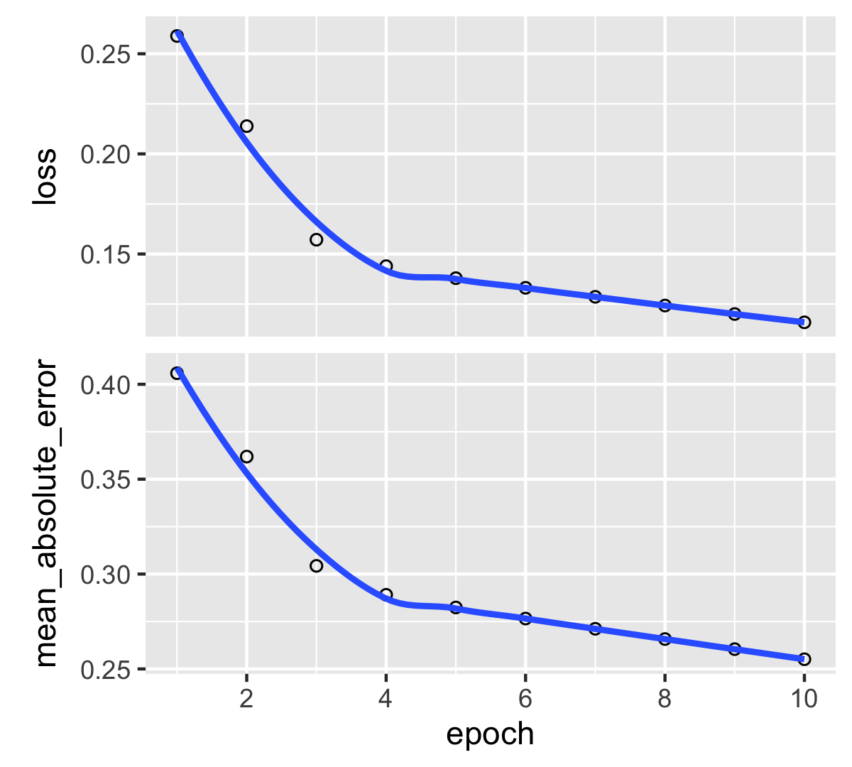

FIGURE 7.10: Output from a trained recurrent neural network (regression task).

Compared to our previous models, the major difference both in the ouptut (the graph on Figure 7.10) and the input (the code) is the absence of validation (or testing) data. One reason for that is because Keras is very restrictive on RNNs and imposes that both the training and testing samples share the same dimensions. In our situation this is obviously not the case, hence we must bypass this obstacle by duplicating the model.

new_model <- keras_model_sequential() %>% 
  layer_gru(units = 16, 
            batch_input_shape = c(nb_stocks,          # New dimensions
                                  nb_dates_test, 
                                  nb_feats), 
            activation = 'tanh',                      # Activation function
            return_sequences = TRUE) %>%              # Return the full sequence
  layer_dense(units = 1)                              # Output dimension
new_model %>% keras::set_weights(keras::get_weights(model_RNN))

Finally, once the new model is ready, and with the matching dimensions, we can push forward to predicting the test values. We resort to the predict() function and immediately compute the hit ratio obtained by the model.

pred_rnn <- predict(new_model, test_features_rnn, batch_size = nb_stocks) # Predictions
mean(c(t(as.matrix(pred_rnn))) * test_labels_rnn > 0)           # Hit ratio

## [1] 0.5007738

The hit ratio is close to 50%, hence the model does hardly better than coin tossing.

Before we close this section on RNNs, we mention a new type architecture, called \(\alpha\)-RNN which are simpler compared to LSTMs and GRUs. They consist in vanilla RNNs to which a simple autocorrelation is added to generate long term memory. We refer to the paper Matthew F. Dixon (2020) for more details on this subject.

7.6 Tabular networks (TabNets)

The superiority of neural networks in tasks related to computer vision and natural language processing is now well established. However, in many ML tournaments in the 2010 decade, neural networks have often been surpassed by tree-based models when dealing with tabular data (see Shwartz-Ziv and Armon (2021)). This puzzle encouraged researchers to construct novel NN structures that are better suited to tabular databases. Examples include Arik and Pfister (2020) and Popov, Morozov, and Babenko (2019). Surprisingly, the reverse idea also exists: Nuti, Rugama, and Thommen (2019) try to adapt trees and random forests so that they behave more like neural networks. The interested reader can have a look at the original papers. In this subsection, we detail the architecture introduced in Arik and Pfister (2020), the so-called TabNets. Even if they are quite young, neural networks for tabular data already have their own survey, Borisov et al. (2021) and they are constantly improved (see Gorishniy, Rubachev, and Babenko (2022)).

7.6.1 The zoo of layers

In Figure 7.3, both layers are of the same type. They take a vector of inputs and return a number which is a linear combination of these inputs. In the ML jargon, this type of layer is called “fully connected” (FC). In Keras syntax, they are referred to as “layer_dense”.

There are many other layer types. The recurrent layer described in the previous section 7.5 is one example and convolutional layers (see next section 7.7.3) are another family of layers. One simple yet useful layer is batch normalization (BN). The idea is that before processing the output of a previous layer, we want to normalize the information that is coming to a new layer. In most of our applications, the inputs and outputs are matrices and BN amounts to perform the same two operations on the columns of these matrices. the first operation is to retrieve the mean, so that column averages are zero. The second operation is to divide by the standard deviation, so that column variances are equal to one. One useful property is that then all inputs have relatively similar statistical properties (though not necessarily the same distributions).

In ML papers, models and architectures are thus represented as series of layers. In short, Figure 7.3 could be written: \[\text{input} \rightarrow FC \rightarrow FC \rightarrow \text{output},\]

which has the advantage of being compact, but which also omits some important details, like the numbers of units per layer and the nature of the activation functions. Modern deep learning models are so complex that succinct overviews like this one are easier to read.

Another interesting layer type is the Gated Linear Unit (GLU). Given a matrix input \(\textbf{X}\), the GLU yields \[\text{GLU}(\textbf{X}) = (\textbf{XW} + \textbf{b}) \cdot \sigma(\textbf{XW} + \textbf{b}),\] where “\(\cdot\)” is the Hadamard (element-wise) matrix product and \(\sigma\) is the sigmoid function (GLUs can be generalized to other easily differentiable functions).

7.6.2 Sparsemax activation

Before we proceed to a direct presentation of TabNets, we need to present an interesting concept introduced by Martins and Astudillo (2016): the sparsemax transform. The original idea of sparsemax is to simplify the softmax activation function for multiclass outputs. At the final stage of a classification network (see Section 7.2.4), the activation is often taken to be \(e^{x_i}/\sum_{j=1}^Je^{x_j}\), where the vector \(\textbf{x}\) is the output of the final layer. Because of the property of the exponential function, this means that all classes will end up with a strictly positive score or probability. This is not desirable because often we prefer decisions that are clear-cut, i.e., when an improbable class gets a zero probability.

To force weak values to zeros, Martins and Astudillo (2016) resort to a special projection which they call sparsemax. The starting point is the \(N-1\)-dimensional simplex

\[ \mathbb{S}_N=\left\{ \mathbf{x} \in \mathbb{R}^N \left|\sum_{n=1}^Nx_n=1, \ x_n\ge 0, \ \forall n=1,\dots N.\right.\right\} \] This space encompasses all possible combinations of probabilities for a classification outcome with \(N\) classes. Given a vector \(\textbf{x}\), the sparsemax function is defined as \[\text{sparsemax}(\textbf{x}) = \underset{\textbf{z} \in \mathbb{S}_N}{\text{argmin}} \ ||\textbf{z} - \textbf{x}||,\] which is equal to the projection of \(\textbf{x}\) onto \(\mathbb{S}_N\). We illustrate the difference between softmax and sparsemax functions in dimension 1 in Figure 7.11. It is clear that the outcome is much clearer for the sparsemax function: when the input is small, the output is zero and when it is large, the output in one. This generates discrepancies that are easier to handle. In large dimension, this yields sparse outputs, which have desirable properties (smaller encoding sizes, simpler interpretation).

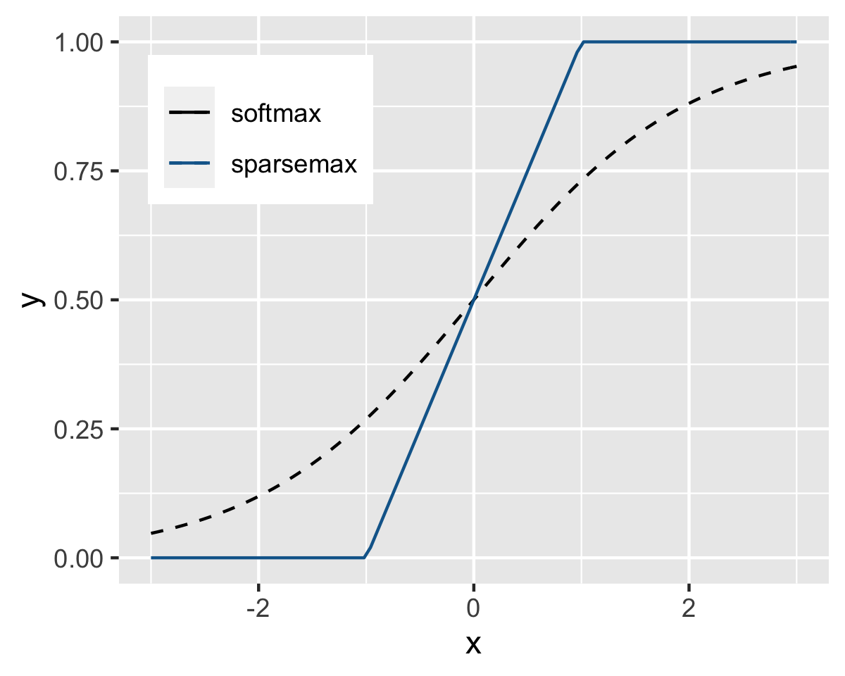
FIGURE 7.11: Softmax versus sparsemax in 1 dimension.

7.6.3 Feature selection

One key element in TabNets is the fact that they are, so to speak “one-size fits all” (akin to Auto-ML, they aim at providing a packaged solution that can tackle a large spectrum of problems.). This is why the batch normalization layers are to useful: they can handle very different type of numerical inputs.

The first important component of TabNets is feature selection. The rationale is that we want to learn more intensely from the predictors which matter and not lose time on noisy variables. As is customary for “vanilla” NNs, we consider the case of a rectangular (matrix-shaped) batch \(\textbf{f}\) of size \(B \times K\). In TabNets, the selection of features takes the form of a mask, that is, another matrix of the same dimension that multiplies (i.e., discounts) its values. If the mask value for an element is 1, the feature remains, if it is zero, it disappears (metaphorically speaking), and in between the two, its important is simply attenuated.

In TabNets, learning is sequential and consists of step. Each step indexed by \(i\). The mask applied to features at step \(i\) is \(\textbf{M}[i]\), so that masked features are \(\textbf{M}[i] \cdot \textbf{f}\), where again \(\cdot\) denotes the Hadamard product.

[To be completed]

7.6.4 The full architecture

[Under construction]

7.6.5 Code and results

In R, TabNets are coded via the torch framework. They require both packages torch & tabnet to be installed. We start by defining the network structure, i.e., setting the hyperparameters. We also resort to the package parsnip from the tidymodels suite, which allows a uniform grammar in model declaration.

if(!require(torch)){install.packages(c("torch", "tabnet"))}
library(torch)          # General framework for NNs
library(tabnet)         # Package for tabular networks
library(recipes)        # Uniform ML models
library(parsnip)
set.seed(42)            # Random seed

tab_model <- tabnet(
  mode = "regression",  # ML task
  epochs = 5,           # Nb epochs / rounds
  batch_size = 4000,    # Batch size
  virtual_batch_size = 1024,
  penalty = 1,
  learn_rate = 0.01,
  decision_width = 16,
  attention_width = 8,
  num_independent = 1,
  num_shared = 1,
  num_steps = 5,
  momentum = 0.02
) %>%
  set_engine("torch") 

Next, we provide the features and label required to learn. We train it on a smaller dataset for simplicity. Note that the syntax is the same as that of simple models in R (e.g., generalized linear models).

data_short <- data_ml %>%         # Shorter dataset
  filter(stock_id %in% stock_ids_short,
         date < "2010-01-01") %>%
  dplyr::select(c("stock_id", "date", features_short, "R1M_Usd"))

fit_tabnet <- tab_model %>%
  fit(R1M_Usd ~ Div_Yld + Eps + Mkt_Cap_12M_Usd + Mom_11M_Usd + Pb + Vol1Y_Usd, 
      data = data_short)   

Finally, we make some predictions and compute the hit ratio.

tab_pred <- predict(fit_tabnet,
                    data_ml %>%                                                # A test set
                      dplyr::filter(stock_id %in% stock_ids_short,
                                    date > "2010-01-01") %>%
                      dplyr::select(c("stock_id", "date", features_short, "R1M_Usd"))) 
mean((data_ml %>%                                                # A test set
  dplyr::filter(stock_id %in% stock_ids_short,
                date > "2010-01-01") %>% 
  pull(R1M_Usd)) * tab_pred > 0)

## [1] 0.5061184

7.7 Other common architectures

In this section, we present other network structures. Because they are less mainstream and often harder to implement, we do not propose code examples and stick to theoretical introductions.

7.7.1 Generative adversarial networks

The idea of Generative Adversarial Networks (GANs) is to improve the accuracy of a classical neural network by trying to fool it. This very popular idea was introduced by Goodfellow et al. (2014). Imagine you are an expert in Picasso paintings and that you boast about being able to easily recognize any piece of work from the painter. One way to refine your skill is to test them against a counterfeiter. A true expert should be able to discriminate between a true original Picasso and one emanating from a forger. This is the principle of GANs.

GANs consist in two neural networks: the first one tries to learn and the second one tries to fool the first (induce it into error). Just like in the example above, there are also two sets of data: one (\(\textbf{x}\)) is true (or correct), stemming from a classical training sample and the other one (\(\textbf{z}\)) is fake and generated by the counterfeiter network.

In the GAN nomenclature, the network that learns is \(D\) because it is supposed to discriminate, while the forger is \(G\) because it generates false data. In their original formulation, GANs are aimed at classifying. To ease the presentation, we keep this scope. The discriminant network has a simple (scalar) output: the probability that its input comes from true data (versus fake data). The input of \(G\) is some arbitrary noise and its output has the same shape/form as the input of \(D\).

We state the theoretical formula of a GAN directly and comment on it below. \(D\) and \(G\) play the following minimax game: \[\begin{equation} \tag{7.7} \underset{G}{\min} \ \underset{D}{\max} \ \left\{ \mathbb{E}[\log(D(\textbf{x}))]+\mathbb{E}[\log(1-D(G(\textbf{z})))] \right\}. \end{equation}\]

First, let us decompose this expression in its two parts (the optimizers). The first part (i.e., the first max) is the classical one: the algorithm seeks to maximize the probability of assigning the correct label to all examples it seeks to classify. As is done in economics and finance, the program does not maximize \(D(\textbf{x})\) itself on average, but rather a functional form (like a utility function).

On the left side, since the expectation is driven by \(\textbf{x}\), the objective must be increasing in the output. On the right side, where the expectation is evaluated over the fake instances, the right classification is the opposite, i.e., \(1-D(G(\textbf{z}))\).

The second, overarching, part seeks to minimize the performance of the algorithm on the simulated data: it aims at shrinking the odds that \(D\) finds out that the data is indeed corrupt. A summarized version of the structure of the network is provided below in Figure (7.8).

\[\begin{equation} \tag{7.8} \left. \begin{array}{rlll} \text{training sample} = \textbf{x} = \text{true data} && \\ \text{noise}= \textbf{z} \quad \overset{G}{\rightarrow} \quad \text{fake data} & \end{array} \right\} \overset{D}{\rightarrow} \text{output = probability for label} \end{equation}\]

In ML-based asset pricing, the most notable application of GANs was introduced in Luyang Chen, Pelger, and Zhu (2020). Their aim is to make use of the method of moment expression \[\mathbb{E}[M_{t+1}r_{t+1,n}g(I_t,I_{t,n})]=0,\] which is an application of Equation (3.7) where the instrumental variables \(I_{t,n}\) are firm-dependent (e.g., characteristics and attributes) while the \(I_t\) are macro-economic variables (aggregate dividend yield, volatility level, credit spread, term spread, etc.). The function \(g\) yields a \(d\)-dimensional output, so that the above equation leads to \(d\) moment conditions. The trick is to model the SDF as an unknown combination of assets \(M_{t+1}=1-\sum_{n=1}^Nw(I_t,I_{t,n})r_{t+1,n}\). The primary discriminatory network (\(D\)) is the one that approximates the SDF via the weights \(w(I_t,I_{t,n})\). The secondary generative network is the one that creates the moment condition through \(g(I_t,I_{t,n})\) in the above equation.

The full specification of the network is given by the program: \[\underset{w}{\text{min}} \ \underset{g}{\text{max}} \ \sum_{j=1}^N \left\| \mathbb{E} \left[\left(1-\sum_{n=1}^Nw(I_t,I_{t,n})r_{t+1,n} \right)r_{t+1,j}g(I_t,I_{t,j})\right] \right\|^2,\]

where the \(L^2\) norm applies on the \(d\) values generated via \(g\). The asset pricing equations (moments) are not treated as equalities but as a relationship that is approximated. The network defined by \(\textbf{w}\) is the asset pricing modeler and tries to determine the best possible model, while the network defined by \(\textbf{g}\) seeks to find the worst possible conditions so that the model performs badly. We refer to the original article for the full specification of both networks. In their empirical section, Luyang Chen, Pelger, and Zhu (2020) report that adopting a strong structure driven by asset pricing imperatives add values compared to a pure predictive ‘vanilla’ approach such as the one detailed in Gu, Kelly, and Xiu (2020b). The out-of-sample behavior of decile sorted portfolios (based on the model’s prediction) display a monotonic pattern with respect to the order of the deciles.

GANs can also be used to generate artificial financial data (see Efimov and Xu (2019), Marti (2019), Wiese et al. (2020), Ni et al. (2020), and, relatedly, Buehler et al. (2020)), but this topic is outside the scope of the book.

7.7.2 Autoencoders

In the recent literature, autoencoders (AEs) are used in Huck (2019) (portfolio management), and Gu, Kelly, and Xiu (2020a) (asset pricing).
AEs are a strange family of neural networks because they are classified among non-supervised algorithms. In the supervised jargon, their label is equal to the input. Like GANS, autoencoders consist of two networks, though the structure is very different: the first network encodes the input into some intermediary output (usually called the code), and the second network decodes the code into a modified version of the input.

\[\begin{array}{ccccccccc} \textbf{x} & &\overset{E}{\longrightarrow} && \textbf{z} && \overset{D}{\longrightarrow} && \textbf{x}' \\ \text{input} && \text{encoder} && \text{code} && \text{decoder} && \text{modified input} \end{array}\]

Because autoencoders do not belong to the large family of supervised algorithms, we postpone their presentation to Section 15.2.3.

The article Gu, Kelly, and Xiu (2020a) resorts to the idea of AEs while at the same time augmenting the complexity of their asset pricing model. From the simple specification \(r_t=\boldsymbol{\beta}_{t-1}\textbf{f}_t+e_t\) (we omit asset dependence for notational simplicity), they add the assumptions that the betas depend on firm characteristics, while the factors are possibly nonlinear functions of the returns themselves. The model takes the following form: \[\begin{equation} \tag{7.9} r_{t,i}=\textbf{NN}_{\textbf{beta}}(\textbf{x}_{t-1,i})+\textbf{NN}_{\textbf{factor}}(\textbf{r}_t)+e_{t,i}, \end{equation}\] where \(\textbf{NN}_{\textbf{beta}}\) and \(\textbf{NN}_{\textbf{factor}}\) are two neural networks. The above equation looks like an autoencoder because the returns are both inputs and outputs. However, the additional complexity comes from the second neural network \(\textbf{NN}_{\textbf{beta}}\). Modern neural network libraries such as Keras allow for customized models like the one above. The coding of this structure is left as exercise (see below).

7.7.3 A word on convolutional networks

Neural networks gained popularity during the 2010 decade thanks to a series of successes in computer vision competitions. The algorithms behind these advances are convolutional neural networks (CNNs). While they may seem a surprising choice for financial predictions, several teams of researchers in the Computer Science field have proposed approaches that rely on this variation of neural networks (J.-F. Chen et al. (2016), Loreggia et al. (2016), Dingli and Fournier (2017), Tsantekidis et al. (2017), Hoseinzade and Haratizadeh (2019)). Recently, J. Jiang, Kelly, and Xiu (2020) propose to extract signals from images of price trends. Hence, we briefly present the principle in this final section on neural networks. We lay out the presentation for CNNs of dimension two, but they can also be used in dimension one or three.

The reason why CNNs are useful is because they allow to progressively reduce the dimension of a large dataset by keeping local information. An image is a rectangle of pixels. Each pixel is usually coded via three layers, one for each color: red, blue and green. But to keep things simple, let’s just consider one layer of, say 1,000 by 1,000 pixels, with one value for each pixel. In order to analyze the content of this image, a convolutional layer will reduce the dimension of inputs by resorting to some convolution. Visually, this simplification is performed by scanning and altering the values using rectangles with arbitrary weights.

Figure 7.12 sketches this process (it is strongly inspired by Hoseinzade and Haratizadeh (2019)). The original data is a matrix \((I\times K)\) \(x_{i,k}\) and the weights are also a matrix \(w_{j,l}\) of size \((J\times L)\) with \(J<I\) and \(L<K\). The scanning transforms each rectangle of size \((J\times L)\) into one real number. Hence, the output has a smaller size: \((I-J+1)\times(K-L+1)\). If \(I=K=1,000\) and \(J=L=201\), then the output has dimension \((800\times 800)\) which is already much smaller. The output values are given by \[o_{i,k}=\sum_{j=1}^J\sum_{l=1}^Lw_{j,l}x_{i+j-1,k+l-1}.\]

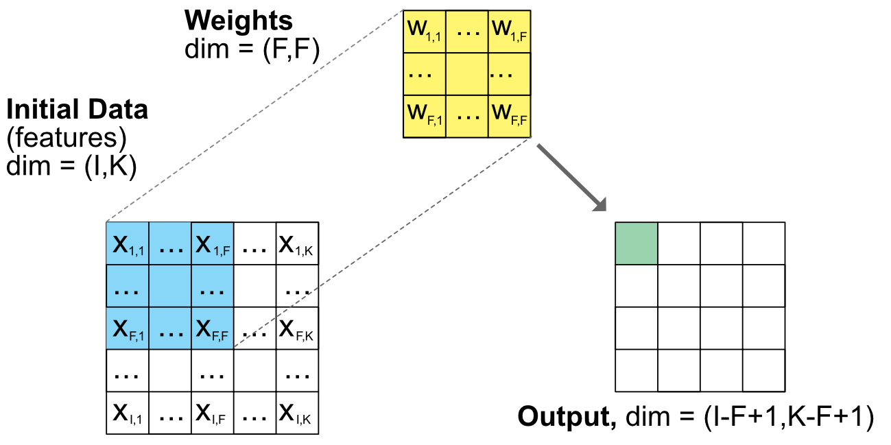
FIGURE 7.12: Scheme of a convolutional unit. Note: the dimensions are general and do not correspond to the number of squares.

Iteratively reducing the dimension of the output via sequences of convolutional layers like the one presented above would be costly in computation and could give rise to overfitting because the number of weights would be incredibly large. In order to efficiently reduce the size of outputs, pooling layers are often used. The job of pooling units is to simplify matrices by reducing them to a simple metric such as the minimum, maximum or average value of the matrix:

\[o_{i,k}=f(x_{i+j-1,k+l-1}, 1\le j\le J, 1 \le l\le L),\]

where \(f\) is the minimum, maximum or average value. We show examples of pooling in Figure 7.13 below. In order to increase the speed of compression, it is possible to add a stride to omit cells. A stride value of \(v\) will perform the operation only every \(v\) value and hence bypass intermediate steps. In Figure 7.13, the two cases on the left do not resort to pooling, hence the reduction in dimension is exactly equal to the size of the pooling size. When stride is into action (right pane), the reduction is more marked. From a 1,000 by 1,000 input, a 2-by-2 pooling layer with stride 2 will yield a 500-by-500 output: the dimension is shrinked fourfold, as in the right scheme of Figure 7.13.

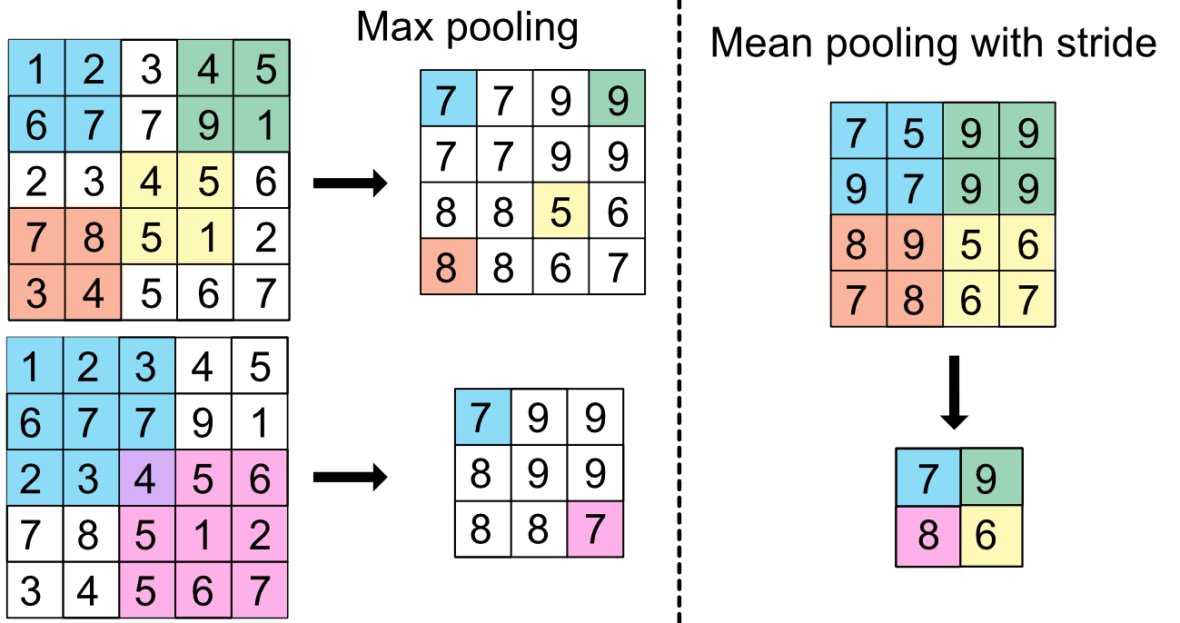
FIGURE 7.13: Scheme of pooling units.

With these tools in hand, it is possible to build new predictive tools. In Hoseinzade and Haratizadeh (2019), predictors such as price quotes, technical indicators and macro-economic data are fed to a complex neural network with 6 layers in order to predict the sign of price variations. While this is clearly an interesting computer science exercise, the deep economic motivation behind this choice of architecture remains unclear. Sangadiev et al. (2020) use CNN to build portfolios relying on limit order book data.

7.8 Coding exercises

1. The purpose of the exercise is to code the autoencoder model described in Gu, Kelly, and Xiu (2020a) (see Section 7.7.2). When coding NNs, the dimensions must be rigorously reported. This is why we reproduce a diagram of the model in Figure 7.14 which clearly shows the inputs and outputs along with their dimensions.

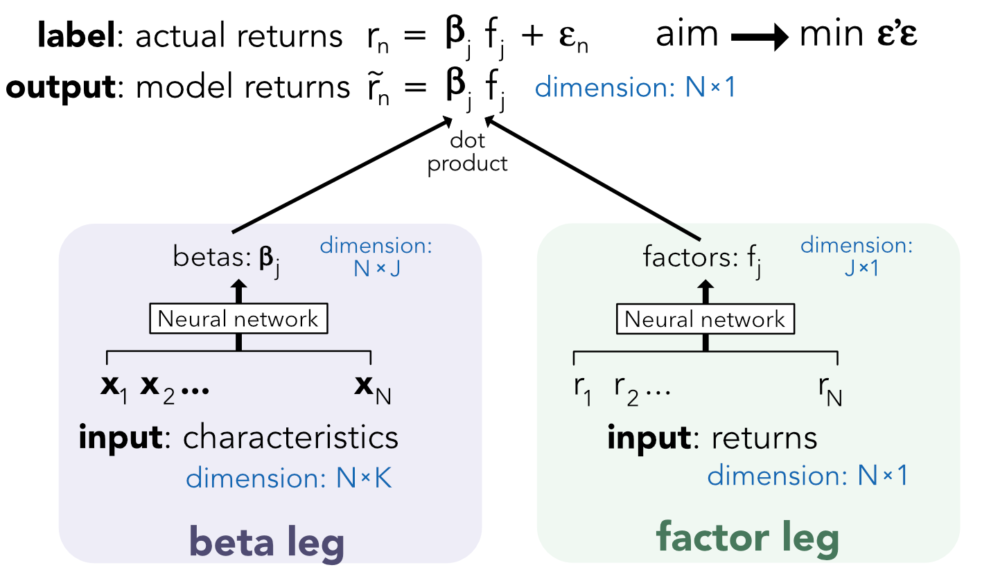
FIGURE 7.14: Scheme of the autoencoder pricing model.

In order to harness the full potential of Keras, it is imperative to switch to more general formulations of NNs. This can be done via the so-called functional API: https://keras.rstudio.com/articles/functional_api.html.

2. The purpose of the exercise is to demonstrate the universal approximation of simple NNs. Let’s take a simple function, say sin(x) over the interval [0,6]. Use a simple feed-forward neural network with one layer and 16 units to mimic this function. Then try with 128 units and see how it improves the fit.

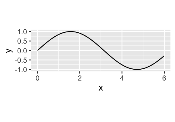
FIGURE 7.15: Goal: approximate this simple function.