 FIGURE 11.1: Scheme of stacked ensembles.
Let us be honest. When facing a prediction task, it is not obvious to determine the best choice between ML tools: penalized regressions, tree methods, neural networks, SVMs, etc. A natural and tempting alternative is to combine several algorithms (or the predictions that result from them) to try to extract value out of each engine (or learner). This intention is not new and contributions towards this goal go back at least to Bates and Granger (1969) (for the purpose of passenger flow forecasting).
Below, we outline a few books on the topic of ensembles. The latter have many names and synonyms, such as forecast aggregation, model averaging, mixture of experts or prediction combination. The first four references below are monographs, while the last two are compilations of contributions:
In this chapter, we cover the basic ideas and concepts behind the notion of ensembles. We refer to the above books for deeper treatments on the topic. We underline that several ensemble methods have already been mentioned and covered earlier, notably in Chapter 6. Indeed, random forests and boosted trees are examples of ensembles. Hence, other early articles on the combination of learners are Schapire (1990), Jacobs et al. (1991) (for neural networks particularly), and Freund and Schapire (1997). Ensembles can for instance be used to aggregate models that are built on different datasets (Pesaran and Pick (2011)), and can be made time-dependent (Sun et al. (2020)). For a theoretical view on ensembles with a Bayesian perspective, we refer to Razin and Levy (2020). Finally, perspectives linked to asset pricing and factor modelling are provided in Gospodinov and Maasoumi (2020) and De Nard, Hediger, and Leippold (2020) (subsampling and forecast aggregation).
In this chapter we adopt the following notations. We work with $M$ models where $\tilde{y}_{i,m}$ is the prediction of model $m$ for instance $i$ and errors $\epsilon_{i,m}=y_i-\tilde{y}_{i,m}$ are stacked into a $(I\times M)$ matrix $\mathbf{E}$. A linear combination of models has sample errors equal to $\textbf{Ew}$, where $\textbf{w}=w_m$ are the weights assigned to each model and we assume $\textbf{w}'\textbf{1}_M=1$. Minimizing the total (squared) error is thus a simple quadratic program with unique constraint. The Lagrange function is $\textbf{w}'\textbf{1}_M=1$ and hence
and the constraint imposes $\textbf{w}^*=\frac{(\textbf{E}'\textbf{E})^{-1}\textbf{1}_M}{(\textbf{1}_M'\textbf{E}'\textbf{E})^{-1}\textbf{1}_M}$ This form is similar to that of minimum variance portfolios. If errors are unbiased $\textbf{1}_I'\textbf{E}=\textbf{0}_M'$, then $\textbf{E}'\textbf{E}$ is the covariance matrix of errors.
This expression shows an important feature of optimized linear ensembles: they can only add value if the models tell different stories. If two models are redundant, $\textbf{E}'\textbf{E}$ will be close to singular and $\textbf{w}^*$ will arbitrage one against the other in a spurious fashion. This is the exact same problem as when mean-variance portfolios are constituted with highly correlated assets: in this case, diversification fails because when things go wrong, all assets go down. Another problem arises when the number of observations is too small compared to the number of assets so that the covariance matrix of returns is singular. This is not an issue for ensembles because the number of observations will usually be much larger than the number of models ($I>>M$).
In the limit when correlations increase to one, the above formulation becomes highly unstable and ensembles cannot be trusted. One heuristic way to see this is when $M=2$ and
$\textbf{E}'\textbf{E}=\left[ \begin{array}{cc} \sigma_1^2 & \rho\sigma_1\sigma_2 \\ \rho\sigma_1\sigma_2 & \sigma_2^2 \\ \end{array} \right] \quad \Leftrightarrow \quad (\textbf{E}'\textbf{E})^{-1}=\frac{1}{1-\rho^2}\left[ \begin{array}{cc} \sigma_1^{-2} & -\rho(\sigma_1\sigma_2)^{-1} \\ -\rho(\sigma_1\sigma_2)^{-1} & \sigma_2^{-2} \\ \end{array} \right]$
so that when $\rho \rightarrow 1$, the model with the smallest errors (minimum $\sigma_i^2$) will see its weight increasing towards infinity while the other model will have a similarly large negative weight: the model arbitrages between two highly correlated variables. This seems like a very bad idea.
There is another illustration of the issues caused by correlations. Let’s assume we face $M$ correlated errors $\epsilon_m$ with pairwise correlation $\rho$ , zero mean and variance $\sigma^2$. The variance of errors is
where while the second term converges to zero as $M$ increases, the first term remains and is linearly increasing with $\rho$ . In passing, because variances are always positive, this result implies that the common pairwise correlation between $M$ variables is bounded below by $-(M-1)^{-1}$. This result is interesting but rarely found in textbooks.
One improvement proposed to circumvent the trouble caused by correlations, advocated in a seminal publication (Breiman (1996)), is to enforce positivity constraints on the weights and solve
Mechanically, if several models are highly correlated, the constraint will impose that only one of them will have a nonzero weight. If there are many models, then just a few of them will be selected by the minimization program. In the context of portfolio optimization, Jagannathan and Ma (2003) have shown the counter-intuitive benefits of constraints in the construction of mean-variance allocations. In our setting, the constraint will similarly help discriminate wisely among the ‘best’ models.
In the literature, forecast combination and model averaging (which are synonyms of ensembles) have been tested on stock markets as early as in Von Holstein (1972). Surprisingly, the articles were not published in Finance journals but rather in fields such as Management (Virtanen and Yli-Olli (1987), Wang et al. (2012)), Economics and Econometrics (Donaldson and Kamstra (1996), Clark and McCracken (2009), Mascio, Fabozzi, and Zumwalt (2020)), Operations Reasearch (Huang, Nakamori, and Wang (2005), Leung, Daouk, and Chen (2001), and Bonaccolto and Paterlini (2019)), and Computer Science (Harrald and Kamstra (1997), Hassan, Nath, and Kirley (2007)).
In the general forecasting literature, many alternative (refined) methods for combining forecasts have been studied. Trimmed opinion pools (Grushka-Cockayne, Jose, and Lichtendahl Jr (2016)) compute averages over the predictions that are not too extreme. Ensembles with weights that depend on previous past errors are developed in Pike and Vazquez-Grande (2020). We refer to Gaba, Tsetlin, and Winkler (2017) for a more exhaustive list of combinations as well as for an empirical study of their respective efficiency. Finally, for a theoretical discussion on model averaging versus model selection, we point to Peng and Yang (2021). Overall, findings are mixed and the heuristic simple average is, as usual, hard to beat (see, e.g., Genre et al. (2013)).
In order to build an ensemble, we must gather the predictions and the corresponding errors into the $\mathbf{E}$ matrix. We will work with 5 models that were trained in the previous chapters: penalized regression, simple tree, random forest, xgboost and feed-forward neural network. The training errors have zero means, hence $\textbf{E}'\textbf{E}$ is the covariance matrix of errors between models.
import pandas as pd
import numpy as np
err_pen_train = fit_pen_pred.predict(X_penalized_train)-training_sample['R1M_Usd']          # Reg.
err_tree_train = fit_tree.predict(training_sample[features])-training_sample['R1M_Usd']     # Tree
err_RF_train = fit_RF.predict(training_sample[features])-training_sample['R1M_Usd']         # RF
err_XGB_train = fit_xgb.predict(train_matrix_xgb)-training_sample['R1M_Usd']                # XGBoost
err_NN_train = model_NN.predict(training_sample[features_short])-training_sample['R1M_Usd'].values.reshape((-1,1))  # NN
E= pd.concat([err_pen_train, err_tree_train,err_RF_train,err_XGB_train,pd.DataFrame(err_NN_train)], axis=1)   # E matrix
E.set_axis(['Pen_reg','Tree','RF','XGB','NN'], axis=1, inplace=True)                            # Names
E.corr()                                                                                        # Cor. mat.
| Pen_reg | Tree | RF | XGB | NN | |
|---|---|---|---|---|---|
| Pen_reg | 1.000000 | 0.998439 | 0.989132 | 0.982260 | 0.998416 |
| Tree | 0.998439 | 1.000000 | 0.990692 | 0.984177 | 0.998498 |
| RF | 0.989132 | 0.990692 | 1.000000 | 0.978393 | 0.990739 |
| XGB | 0.982260 | 0.984177 | 0.978393 | 1.000000 | 0.984303 |
| NN | 0.998416 | 0.998498 | 0.990739 | 0.984303 | 1.000000 |
E.corr().mean()
Pen_reg    0.993649
Tree       0.994361
RF         0.989791
XGB        0.985826
NN         0.994391
dtype: float64
As is shown by the correlation matrix, the models fail to generate heterogeneity in their predictions. The minimum correlation (though above 95%!) is obtained by the boosted tree models. Below, we compare the training accuracy of models by computing the average absolute value of errors.
abs(E).mean() # Mean absolute error or columns of E
Pen_reg    0.083459
Tree       0.083621
RF         0.074806
XGB        0.084048
NN         0.083627
dtype: float64
The best performing ML engine is the random forest. The boosted tree model is the worst, by far. Below, we compute the optimal (non-constrained) weights for the combination of models.
w_ensemble = np.linalg.inv((E.T.values@E.values))@np.ones(5)                    # Optimal weights
w_ensemble /= np.sum(w_ensemble)
w_ensemble
array([ 1.02220538, -2.22814584, 3.93749133, 0.56469433, -2.29624521])
Because of the high correlations, the optimal weights are not balanced and diversified: they load heavily on the random forest learner (best in sample model) and ‘short’ a few models in order to compensate. As one could expect, the model with the largest negative weights (Pen_reg) has a very high correlation with the random forest algorithm (0.997).
Note that the weights are of course computed with training errors. The optimal combination is then tested on the testing sample. Below, we compute out-of-sample (testing) errors and their average absolute value.
err_pen_test = fit_pen_pred.predict(X_penalized_test)-testing_sample['R1M_Usd']          # Reg.
err_tree_test = fit_tree.predict(testing_sample[features])-testing_sample['R1M_Usd']     # Tree
err_RF_test = fit_RF.predict(testing_sample[features])-testing_sample['R1M_Usd']         # RF
err_XGB_test = fit_xgb.predict(test_matrix_xgb)-testing_sample['R1M_Usd']                # XGBoost
err_NN_test = model_NN.predict(testing_sample[features_short])-testing_sample['R1M_Usd'].values.reshape((-1,1))  # NN
E_test= pd.concat([err_pen_test, err_tree_test,err_RF_test,err_XGB_test,pd.DataFrame(err_NN_test,index=testing_sample.index)], axis=1)   # E_test matrix
E_test.set_axis(['Pen_reg','Tree','RF','XGB','NN'], axis=1, inplace=True)                       # Names
abs(E_test).mean() # Mean absolute error or columns of E_test
Pen_reg    0.066182
Tree       0.066535
RF         0.067986
XGB        0.068569
NN         0.066613
dtype: float64
The boosted tree model is still the worst performing algorithm while the simple models (regression and simple tree) are the ones that fare the best. The most naive combination is the simple average of model and predictions.
err_EW_test = np.mean(np.abs(E_test.mean(axis=1))) # equally weight combination
print(f'equally weight combination: {err_EW_test}')
equally weight combination: 0.06673125663086175
Because the errors are very correlated, the equally weighted combination of forecasts yields an average error which lies ‘in the middle’ of individual errors. The diversification benefits are too small. Let us now test the ‘optimal’ combination $\textbf{w}^*=\frac{(\textbf{E}'\textbf{E})^{-1}\textbf{1}_M}{(\textbf{1}_M'\textbf{E}'\textbf{E})^{-1}\textbf{1}_M}$
err_opt_test =np.mean(np.abs(E_test.values@w_ensemble)) # Optimal unconstrained combination
print(f'Optimal unconstrained combination: {err_opt_test}')
Optimal unconstrained combination: 0.08351002385399925
Again, the result is disappointing because of the lack of diversification across models. The correlations between errors are high not only on the training sample, but also on the testing sample, as shown below.
E_test.corr() # Cor. mat.
| Pen_reg | Tree | RF | XGB | NN | |
|---|---|---|---|---|---|
| Pen_reg | 1.000000 | 0.998707 | 0.991539 | 0.966304 | 0.998564 |
| Tree | 0.998707 | 1.000000 | 0.993818 | 0.968991 | 0.998854 |
| RF | 0.991539 | 0.993818 | 1.000000 | 0.972710 | 0.993923 |
| XGB | 0.966304 | 0.968991 | 0.972710 | 1.000000 | 0.969315 |
| NN | 0.998564 | 0.998854 | 0.993923 | 0.969315 | 1.000000 |
The leverage from the optimal solution only exacerbates the problem and underperforms the heuristic uniform combination. We end this section with the constrained formulation of Breiman (1996) for the quadratic optimisation. If we write $\mathbf{\Sigma}$ for the covariance matrix of errors, we seek
The constraints will be handled as:
where the first line will be an equality (weights sum to one) and the last three will be inequalities (weights are all positive).
from cvxopt import matrix, solvers                    # Library for quadratic programming
sigma = E.T.values@E.values                           # Unscaled covariance matrix
nb_mods= 5                                            # Number of models
Q = 2*matrix(sigma, tc="d")                           # Symmetric quadratic-cost matrix
p = matrix(np.zeros(nb_mods),tc="d")                  # Quadratic-cost vector
G = matrix(-np.eye(nb_mods), tc="d")                  # Linear inequality constraint matrix
h = matrix(np.zeros(nb_mods), tc="d")                 # Linear inequality constraint vector
A = matrix(np.ones(nb_mods), (1, nb_mods))            # matrix for linear equality constraint
b = matrix(1.0)                                       # vector for linear equality constraint
w_const=solvers.qp(Q, p, G, h, A, b)                  # Solution
print(w_const['x']) # Solution
     pcost       dcost       gap    pres   dres
 0:  3.3445e+03  3.3656e+03  5e+01  7e+00  1e+01
 1:  3.3575e+03  3.4486e+03  2e+01  4e+00  6e+00
 2:  3.4155e+03  3.5580e+03  2e+01  2e+00  4e+00
 3:  3.5873e+03  4.1600e+03  3e+02  2e+00  3e+00
 4:  3.9350e+03  4.4186e+03  2e+02  1e+00  2e+00
 5:  5.2828e+03  4.1593e+03  2e+03  8e-01  1e+00
 6:  4.9769e+03  4.6678e+03  3e+02  3e-16  2e-11
 7:  4.7556e+03  4.7111e+03  4e+01  1e-16  3e-12
 8:  4.7238e+03  4.7233e+03  6e-01  1e-16  5e-12
 9:  4.7234e+03  4.7234e+03  6e-03  2e-16  4e-12
10:  4.7234e+03  4.7234e+03  6e-05  4e-16  4e-12
Optimal solution found.
[ 5.66e-09]
[ 5.68e-09]
[ 1.00e+00]
[ 6.34e-08]
[ 5.70e-09]
Compared to the unconstrained solution, the weights are sparse and concentrated in one model, usually the one with small training sample errors.
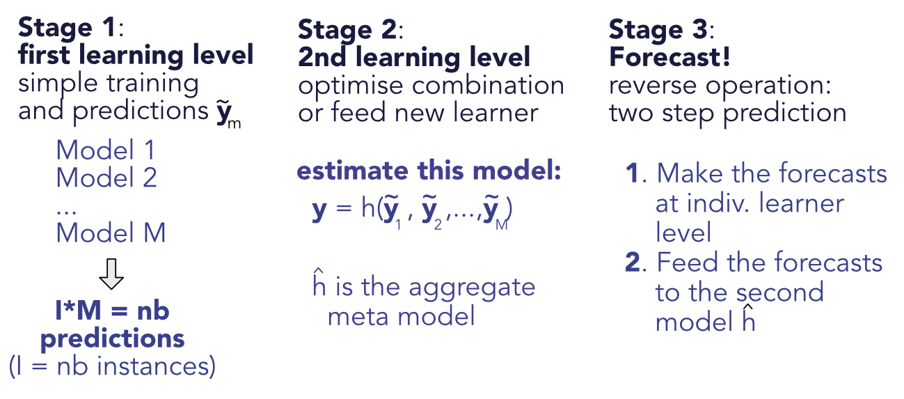
Stacked ensembles are a natural generalization of linear ensembles. The idea of generalizing linear ensembles goes back at least to Wolpert (1992b). In the general case, the training is performed in two stages. The first stage is the simple one, whereby the $M$ models are trained independently, yielding the predictions $\tilde{y}_{i,m}$ for instance $i$ and model $m$. The second step is to consider the output of the trained models as input for a new level of machine learning optimization. The second level predictions are $\breve{y}_i=h(\tilde{y}_{i,1},\dots,\tilde{y}_{i,M})$, where $h$ is a new learner (see Figure 11.1). Linear ensembles are of course stacked ensembles in which the second layer is a linear regression.
The same techniques are then applied to minimize the error between the true values $y_i$ and the predicted ones $\breve{y}_i$.
FIGURE 11.1: Scheme of stacked ensembles.
Below, we create a low-dimensional neural network which takes in the individual predictions of each model and compiles them into a synthetic forecast.
import tensorflow as tf
from tensorflow import keras
from tensorflow.keras import layers
from plot_keras_history import show_history

model_stack = keras.Sequential() # This defines the structure of the network, i.e. how layers are organized
model_stack.add(layers.Dense(8, activation="relu", input_shape=(nb_mods,)))
model_stack.add(layers.Dense(4, activation="tanh"))
model_stack.add(layers.Dense(1))
The configuration is very simple. We do not include any optional arguments and hence the model is likely to overfit. As we seek to predict returns, the loss function is the standard $L^2$ norm.
model_stack.compile(optimizer='RMSprop',                        # Optimisation method (weight updating)
              loss='mse',                                       # Loss function
              metrics=['MeanAbsoluteError'])                    # Output metric
model_stack.summary()                                           # Model architecture
Model: "sequential_1"
_________________________________________________________________
 Layer (type)                Output Shape              Param #
=================================================================
 dense_3 (Dense)             (None, 8)                 48

 dense_4 (Dense)             (None, 4)                 36

 dense_5 (Dense)             (None, 1)                 5

=================================================================
Total params: 89
Trainable params: 89
Non-trainable params: 0
_________________________________________________________________
y_tilde = E.values + np.tile(training_sample['R1M_Usd'].values.reshape(-1, 1), nb_mods)    # Train preds
y_test = E_test.values + np.tile(testing_sample['R1M_Usd'].values.reshape(-1, 1), nb_mods) # Testing
fit_NN_stack  = model_stack.fit(y_tilde,                            # Train features
                          NN_train_labels,                          # Train labels
                          batch_size=512,                           # Train parameters
                          epochs=12,                                # Train parameters
                          verbose=1,                                # Show messages
                          validation_data=(y_test,NN_test_labels))  # Test features & labels
show_history(fit_NN_stack )                                         # Show training plot
Epoch 1/12
387/387 [==============================] - 1s 2ms/step - loss: 0.0213 - mean_absolute_error: 0.0675 - val_loss: 0.0402 - val_mean_absolute_error: 0.0803
Epoch 2/12
387/387 [==============================] - 1s 1ms/step - loss: 0.0191 - mean_absolute_error: 0.0634 - val_loss: 0.0406 - val_mean_absolute_error: 0.0814
Epoch 3/12
387/387 [==============================] - 1s 1ms/step - loss: 0.0188 - mean_absolute_error: 0.0634 - val_loss: 0.0402 - val_mean_absolute_error: 0.0817
Epoch 4/12
387/387 [==============================] - 0s 1ms/step - loss: 0.0186 - mean_absolute_error: 0.0633 - val_loss: 0.0400 - val_mean_absolute_error: 0.0804
Epoch 5/12
387/387 [==============================] - 0s 1ms/step - loss: 0.0186 - mean_absolute_error: 0.0632 - val_loss: 0.0404 - val_mean_absolute_error: 0.0821
Epoch 6/12
387/387 [==============================] - 1s 1ms/step - loss: 0.0184 - mean_absolute_error: 0.0632 - val_loss: 0.0401 - val_mean_absolute_error: 0.0811
Epoch 7/12
387/387 [==============================] - 1s 1ms/step - loss: 0.0183 - mean_absolute_error: 0.0631 - val_loss: 0.0404 - val_mean_absolute_error: 0.0821
Epoch 8/12
387/387 [==============================] - 0s 1ms/step - loss: 0.0183 - mean_absolute_error: 0.0631 - val_loss: 0.0406 - val_mean_absolute_error: 0.0826
Epoch 9/12
387/387 [==============================] - 1s 1ms/step - loss: 0.0181 - mean_absolute_error: 0.0632 - val_loss: 0.0403 - val_mean_absolute_error: 0.0820
Epoch 10/12
387/387 [==============================] - 0s 1ms/step - loss: 0.0181 - mean_absolute_error: 0.0632 - val_loss: 0.0403 - val_mean_absolute_error: 0.0820
Epoch 11/12
387/387 [==============================] - 1s 1ms/step - loss: 0.0181 - mean_absolute_error: 0.0632 - val_loss: 0.0401 - val_mean_absolute_error: 0.0816
Epoch 12/12
387/387 [==============================] - 1s 1ms/step - loss: 0.0181 - mean_absolute_error: 0.0632 - val_loss: 0.0401 - val_mean_absolute_error: 0.0817

FIGURE 11.2: Training metrics for the ensemble model.
The performance of the ensemble is again disappointing: the learning curve is flat in Figure 11.2, hence the rounds of back-propagation are useless. The training adds little value which means that the new overarching layer of ML does not enhance the original predictions. Again, this is because all ML engines seem to be capturing the same patterns and both their linear and non-linear combinations fail to improve their performance.
In a financial context, macro-economic indicators could add value to the process. It is possible that some models perform better under certain conditions and exogenous predictors can help introduce a flavor of economic-driven conditionality in the predictions.
Adding macro-variables to the set of predictors (here, predictions) $\tilde{y}_{i,m}$ could seem like one way to achieve this. However, this would amount to mix predicted values with (possibly scaled) economic indicators and that would not make much sense.
One alternative outside the perimeter of ensembles is to train simple trees on a set of macro-economic indicators. If the labels are the (possibly absolute) errors stemming from the original predictions, then the trees will create clusters of homogeneous error values. This will hint towards which conditions lead to the best and worst forecasts. We test this idea below, using aggregate data from the Federal Reserve of Saint Louis. We download and format the data in the next chunk.
macro_cond = pd.read_csv("macro_cond.csv")                                           # Term Spred, Inflation and Consumer Price Index
macro_cond["Index"] = pd.to_datetime(macro_cond["date"]) + pd.offsets.MonthBegin(-1) # Change date to first day of month to join/merge
ens_data=pd.DataFrame()
ens_data['date'] = testing_sample["date"].values
ens_data['err_NN_test'] = err_NN_test                                        # Using the errors from previous section
ens_data["Index"] = pd.to_datetime(ens_data["date"]) + pd.offsets.MonthBegin(-1)     # Change date to first day of month to join/merge
ens_data = pd.merge(ens_data, macro_cond, how="left", left_on="Index", right_on="Index")
ens_data.head()                                                                      # Show first lines
| date_x | err_NN_test | Index | date_y | CPIAUCSL | inflation | termspread | |
|---|---|---|---|---|---|---|---|
| 0 | 2014-01-31 | 0.084440 | 2014-01-01 | 31/01/2014 | 235.288 | 0.002424 | 2.47 |
| 1 | 2014-01-31 | 0.073821 | 2014-01-01 | 31/01/2014 | 235.288 | 0.002424 | 2.47 |
| 2 | 2014-01-31 | -0.254902 | 2014-01-01 | 31/01/2014 | 235.288 | 0.002424 | 2.47 |
| 3 | 2014-01-31 | 0.266475 | 2014-01-01 | 31/01/2014 | 235.288 | 0.002424 | 2.47 |
| 4 | 2014-01-31 | -0.079414 | 2014-01-01 | 31/01/2014 | 235.288 | 0.002424 | 2.47 |
We can now build a tree that tries to explain the accuracy of models as a function of macro-variables.
X_ens = ens_data[['inflation','termspread']]                                         # Training macro features
y_ens = abs(ens_data['err_NN_test'])                                                 # Label, here error from previous section
fit_ens  = tree.DecisionTreeRegressor(                                               # Definining the model
  max_depth = 2,                                                                     # Maximum depth (i.e. tree levels)
  ccp_alpha=0.00001                                                                  # complexity parameters
        )
fit_ens.fit(X_ens, y_ens)                                                            # Fitting the model
fig, ax = plt.subplots(figsize=(13, 8))                                              # resizing
tree.plot_tree(fit_ens ,feature_names=X_ens.columns.values, ax=ax)                   # Plot the tree
plt.show()

FIGURE 11.3: Conditional performance of a ML engine.
The tree creates clusters which have homogeneous values of absolute errors. One big cluster gathers 80% of predictions (the right one) and is the one with the smallest average. It corresponds to the periods when the term spread is above 0.29 (in percentage points). The other two groups (when the term spread is below 0.29%) are determined according to the level of inflation. If the latter is positive, then the average absolute error is 8%, if not, it is 13%.
As shown earlier in this chapter, one major problem with ensembles arises when the first layer of predictions is highly correlated. In this case, ensembles are pretty much useless. There are several tricks that can help reduce this correlation, but the simplest and best is probably to alter training samples. If algorithms do not see the same data, they will probably infer different patterns.
There are several ways to split the training data so as to build different subsets of training samples. The first dichotomy is between random versus deterministic splits. Random splits are easy and require only the target sample size to be fixed. Note that the training samples can be overlapping as long as the overlap is not too large. Hence if the original training sample has
$I$ instance and the ensemble requires $M$ models, then a subsample size of $\lfloor I/M \rfloor$ may be too conservative especially if the training sample is not very large. In this case $\lfloor I/\sqrt{M} \rfloor$ may be a better alternative. Random forests are one example of ensembles built in random training samples.
One advantage of deterministic splits is that they are easy to reproduce and their outcome does not depend on the random seed. By the nature of factor-based training samples, the second splitting dichotomy is between time and assets. A split within assets is straightforward: each model is trained on a different set of stocks. Note that the choices of sets can be random, or dictacted by some factor-based criterion: size, momentum, book-to-market ratio, etc.
A split in dates requires other decisions: is the data split in large blocks (like years) and each model gets a block, which may stand for one particular kind of market condition? Or are the training dates divided more regularly? For instance, if there are 12 models in the ensemble, each model can be trained on data from a given month (e.g., January for the first models, February for the second, etc.).
Below, we train four models on four different years to see if this helps reduce the inter-model correlations. This process is a bit lengthy because the samples and models need to be all redefined. We start by creating the four training samples. The third model works on the small subset of features, hence the sample is smaller.
training_sample_2007 = training_sample.loc[training_sample.index[(
    training_sample['date'] > '2006-12-31') & (training_sample['date'] < '2008-01-01')].tolist()]
training_sample_2009 = training_sample.loc[training_sample.index[(
    training_sample['date'] > '2008-12-31') & (training_sample['date'] < '2010-01-01')].tolist()]
training_sample_2011 = training_sample.loc[training_sample.index[(
    training_sample['date'] > '2010-12-31') & (training_sample['date'] < '2012-01-01')].tolist()]
training_sample_2013 = training_sample.loc[training_sample.index[(
    training_sample['date'] > '2012-12-31') & (training_sample['date'] < '2014-01-01')].tolist()]
Then, we proceed to the training of the models. The syntaxes are those used in the previous chapters, nothing new here. We start with a penalized regression. In all predictions below, the original testing sample is used for all models.
y_ens_2007 = training_sample_2007['R1M_Usd'].values                                 # Dep. var.
x_ens_2007 = training_sample_2007[features].values                                  # Predictors
model_2007 = ElasticNet(alpha=0.1, l1_ratio=0.1)                                    # Model
fit_ens_2007=model_2007.fit(x_ens_2007,y_ens_2007)                                  # fitting the model
err_ens_2007 = fit_ens_2007.predict(X_penalized_test)-testing_sample['R1M_Usd']     # Pred. errs
We continue with a random forest.
from sklearn.ensemble import RandomForestRegressor
fit_ens_2009 = RandomForestRegressor(n_estimators = 40, # Nb of random trees
criterion ='mse', # function to measure the quality of a split
min_samples_split= 250, # Minimum size of terminal cluster
bootstrap=False, # replacement
max_features=30, # Nb of predictive variables for each tree
max_samples=4000 # Size of (random) sample for each tree
)
fit_ens_2009.fit(training_sample_2009[features].values,training_sample_2009['R1M_Usd'].values ) # Fitting the model
err_ens_2009=fit_ens_2009.predict(pd.DataFrame(X_test))-testing_sample['R1M_Usd'] # Pred. errs
The third model is a boosted tree.
train_features_xgb_2011=training_sample_2011[features_short].values # Independent variables
train_label_xgb_2011=training_sample_2011['R1M_Usd'].values # Dependent variable
train_matrix_xgb_2011=xgb.DMatrix(train_features_xgb_2011, label=train_label_xgb_2011) # XGB format!

params={'eta' : 0.3,                          # Learning rate
  'objective' : "reg:squarederror",     # Objective function
  'max_depth' : 4,                      # Maximum depth of trees
  'subsample' : 0.6,                    # Train on random 60% of sample
  'colsample_bytree' : 0.7,             # Train on random 70% of predictors
  'lambda' : 1,                         # Penalisation of leaf values
  'gamma' : 0.1}                        # Penalisation of number of leaves
fit_ens_2011 =xgb.train(params, train_matrix_xgb_2011, num_boost_round=18) # Number of trees used
err_ens_2011=fit_ens_2011.predict(test_matrix_xgb)-testing_sample['R1M_Usd'] # Pred. errs
Finally, the last model is a simple neural network.
model = keras.Sequential()
model.add(layers.Dense(16, activation="relu", input_shape=(len(features),)))
model.add(layers.Dense(8, activation="tanh"))
model.add(layers.Dense(1))
model.compile(optimizer='RMSprop',
              loss='mse',
              metrics=['MeanAbsoluteError'])
model.summary()
fit_ens_2013 = model.fit(
            training_sample_2013[features].values,                  # Training features
            training_sample_2013['R1M_Usd'].values,                 # Training labels
            batch_size=128,                                         # Training parameters
            epochs = 9,                                             # Training parameters
            verbose = True                                          # Show messages
)

err_ens_2013=model.predict(X_penalized_test)-testing_sample['R1M_Usd'].values.reshape((-1,1)) # Pred. errs
Model: "sequential_2"
_________________________________________________________________
 Layer (type)                Output Shape              Param #
=================================================================
 dense_6 (Dense)             (None, 16)                1504

 dense_7 (Dense)             (None, 8)                 136

 dense_8 (Dense)             (None, 1)                 9

=================================================================
Total params: 1,649
Trainable params: 1,649
Non-trainable params: 0
_________________________________________________________________
Epoch 1/9
112/112 [==============================] - 1s 1ms/step - loss: 0.0253 - mean_absolute_error: 0.1083
Epoch 2/9
112/112 [==============================] - 0s 1ms/step - loss: 0.0075 - mean_absolute_error: 0.0609
Epoch 3/9
112/112 [==============================] - 0s 1ms/step - loss: 0.0072 - mean_absolute_error: 0.0595
Epoch 4/9
112/112 [==============================] - 0s 1ms/step - loss: 0.0072 - mean_absolute_error: 0.0594
Epoch 5/9
112/112 [==============================] - 0s 1ms/step - loss: 0.0072 - mean_absolute_error: 0.0594
Epoch 6/9
112/112 [==============================] - 0s 1ms/step - loss: 0.0071 - mean_absolute_error: 0.0593
Epoch 7/9
112/112 [==============================] - 0s 1ms/step - loss: 0.0071 - mean_absolute_error: 0.0593
Epoch 8/9
112/112 [==============================] - 0s 1ms/step - loss: 0.0071 - mean_absolute_error: 0.0593
Epoch 9/9
112/112 [==============================] - 0s 1ms/step - loss: 0.0071 - mean_absolute_error: 0.0591
Endowed with the errors of the four models, we can compute their correlation matrix.
E_subtraining = pd.concat([err_ens_2007, err_ens_2009,err_ens_2011,pd.DataFrame(err_ens_2013,index=testing_sample.index)], axis=1)         # E_subtraining matrix
E_subtraining.set_axis(['err_ens_2007','err_ens_2009','err_ens_2011','err_ens_2013'], axis=1, inplace=True)   # Names
E_subtraining.corr()
| err_ens_2007 | err_ens_2009 | err_ens_2011 | err_ens_2013 | |
|---|---|---|---|---|
| err_ens_2007 | 1.000000 | 0.953756 | 0.868026 | 0.998962 |
| err_ens_2009 | 0.953756 | 1.000000 | 0.842201 | 0.955961 |
| err_ens_2011 | 0.868026 | 0.842201 | 1.000000 | 0.868046 |
| err_ens_2013 | 0.998962 | 0.955961 | 0.868046 | 1.000000 |
E_subtraining.corr().mean()
err_ens_2007    0.955186
err_ens_2009    0.937980
err_ens_2011    0.894568
err_ens_2013    0.955742
dtype: float64
The results are overall disappointing. Only one model manages to extract patterns that are somewhat different from the other ones, resulting in a 89% correlation across the board. Neural networks (on 2013 data) and penalized regressions (2007) remain highly correlated. One possible explanation could be that the models capture mainly noise and little signal. Working with long-term labels like annual returns could help improve diversification across models.
Build an integrated ensemble on top of 3 neural networks trained entirely with Keras. Each network obtains one third of predictors as input. The three networks yield a classification (yes/no or buy/sell). The overarching network aggregates the three outputs into a final decision. Evaluate its performance on the testing sample. Use the functional API.
Bates, John M, and Clive WJ Granger. 1969. “The Combination of Forecasts.” Journal of the Operational Research Society 20 (4): 451–68.
Bonaccolto, Giovanni, and Sandra Paterlini. 2019. “Developing New Portfolio Strategies by Aggregation.” Annals of Operations Research, 1–39.
Breiman, Leo. 1996. “Stacked Regressions.” Machine Learning 24 (1): 49–64.
Claeskens, Gerda, and Nils Lid Hjort. 2008. Model Selection and Model Averaging. Cambridge University Press.
Clark, Todd E, and Michael W McCracken. 2009. “Improving Forecast Accuracy by Combining Recursive and Rolling Forecasts.” International Economic Review 50 (2): 363–95.
De Nard, Gianluca, Simon Hediger, and Markus Leippold. 2020. “Subsampled Factor Models for Asset Pricing: The Rise of Vasa.” SSRN Working Paper 3557957.
Donaldson, R Glen, and Mark Kamstra. 1996. “Forecast Combining with Neural Networks.” Journal of Forecasting 15 (1): 49–61.
Freund, Yoav, and Robert E Schapire. 1997. “A Decision-Theoretic Generalization of on-Line Learning and an Application to Boosting.” Journal of Computer and System Sciences 55 (1): 119–39.
Gaba, Anil, Ilia Tsetlin, and Robert L Winkler. 2017. “Combining Interval Forecasts.” Decision Analysis 14 (1): 1–20.
Genre, Véronique, Geoff Kenny, Aidan Meyler, and Allan Timmermann. 2013. “Combining Expert Forecasts: Can Anything Beat the Simple Average?” International Journal of Forecasting 29 (1): 108–21.
Gospodinov, Nikolay, and Esfandiar Maasoumi. 2020. “Generalized Aggregation of Misspecified Models: With an Application to Asset Pricing.” Journal of Econometrics Forthcoming.
Grushka-Cockayne, Yael, Victor Richmond R Jose, and Kenneth C Lichtendahl Jr. 2016. “Ensembles of Overfit and Overconfident Forecasts.” Management Science 63 (4): 1110–30.
Harrald, Paul G, and Mark Kamstra. 1997. “Evolving Artificial Neural Networks to Combine Financial Forecasts.” IEEE Transactions on Evolutionary Computation 1 (1): 40–52.
Hassan, Md Rafiul, Baikunth Nath, and Michael Kirley. 2007. “A Fusion Model of Hmm, Ann and Ga for Stock Market Forecasting.” Expert Systems with Applications 33 (1): 171–80.
Huang, Wei, Yoshiteru Nakamori, and Shou-Yang Wang. 2005. “Forecasting Stock Market Movement Direction with Support Vector Machine.” Computers & Operations Research 32 (10): 2513–22.
Jacobs, Robert A, Michael I Jordan, Steven J Nowlan, Geoffrey E Hinton, and others. 1991. “Adaptive Mixtures of Local Experts.” Neural Computation 3 (1): 79–87.
Jagannathan, Ravi, and Tongshu Ma. 2003. “Risk Reduction in Large Portfolios: Why Imposing the Wrong Constraints Helps.” Journal of Finance 58 (4): 1651–83.
Leung, Mark T, Hazem Daouk, and An-Sing Chen. 2001. “Using Investment Portfolio Return to Combine Forecasts: A Multiobjective Approach.” European Journal of Operational Research 134 (1): 84–102.
Mascio, David A, Frank J Fabozzi, and J Kenton Zumwalt. 2020. “Market Timing Using Combined Forecasts and Machine Learning.” Journal of Forecasting Forthcoming.
Okun, Oleg, Giorgio Valentini, and Matteo Re. 2011. Ensembles in Machine Learning Applications. Vol. 373. Springer Science & Business Media.
Peng, Jingfu, and Yuhong Yang. 2021. “On Improvability of Model Selection by Model Averaging.” Journal of Econometrics Forthcoming.
Pesaran, M Hashem, and Andreas Pick. 2011. “Forecast Combination Across Estimation Windows.” Journal of Business & Economic Statistics 29 (2): 307–18.
Pike, Tyler, and Francisco Vazquez-Grande. 2020. “Combining Forecasts: Can Machines Beat the Average?” SSRN Working Paper 3691117.
Razin, Ronny, and Gilat Levy. 2020. “A Maximum Likelihood Approach to Combining Forecasts.” Theoretical Economics Forthcoming.
Schapire, Robert E. 1990. “The Strength of Weak Learnability.” Machine Learning 5 (2): 197–227.
Schapire, Robert E, and Yoav Freund. 2012. Boosting: Foundations and Algorithms. MIT Press.
Seni, Giovanni, and John F Elder. 2010. “Ensemble Methods in Data Mining: Improving Accuracy Through Combining Predictions.” Synthesis Lectures on Data Mining and Knowledge Discovery 2 (1): 1–126.
Sun, Yuying, YM Hong, T Lee, Shouyang Wang, and Xinyu Zhang. 2020. “Time-Varying Model Averaging.” Journal of Econometrics Forthcoming.
Virtanen, Ilkka, and Paavo Yli-Olli. 1987. “Forecasting Stock Market Prices in a Thin Security Market.” Omega 15 (2): 145–55.
Von Holstein, Carl-Axel S Staël. 1972. “Probabilistic Forecasting: An Experiment Related to the Stock Market.” Organizational Behavior and Human Performance 8 (1): 139–58.
Wang, Ju-Jie, Jian-Zhou Wang, Zhe-George Zhang, and Shu-Po Guo. 2012. “Stock Index Forecasting Based on a Hybrid Model.” Omega 40 (6): 758–66.
Wolpert, David H. 1992b. “Stacked Generalization.” Neural Networks 5 (2): 241–59.
Zhang, Cha, and Yunqian Ma. 2012. Ensemble Machine Learning: Methods and Applications. Springer.
Zhou, Zhi-Hua. 2012. Ensemble Methods: Foundations and Algorithms. Chapman & Hall / CRC.